The Jump Strategy

Big Idea

We can express any finitely-changing step function $f(t)$ in terms of unit-step functions using the following strategy.

$f(t) = (\text{start}) + (\text{jump}_1) \cdot U(t - t_1) + (\text{jump}_2) \cdot U(t - t_2) + \cdots.$

For a complete derivation, see this post. Computing Laplace transforms becomes trivial since $\mathcal L\{\cdot\}$ is linear and $\mathcal L\{U(t-a)\} = e^{-as}/s$ . Recall that the unit step function is defined by

$U(t-a) := \begin{cases} 0, & t < a, \\ 1, & t \geq a. \end{cases}$

Questions

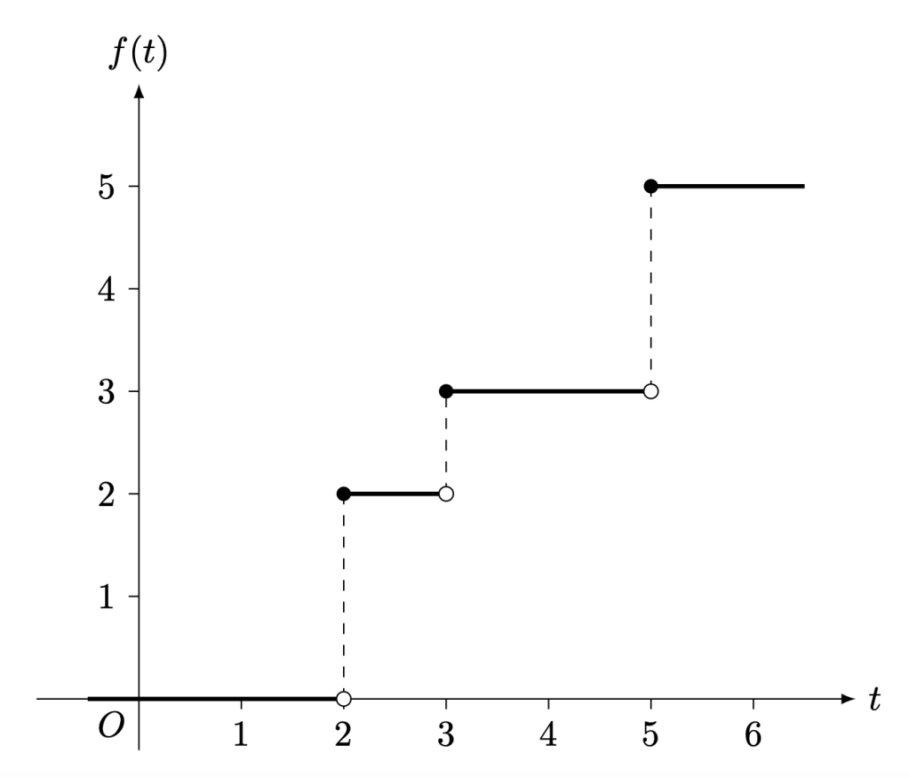
Question 1. The function $f$ is defined by the graph below.

Evaluate $\mathcal L\{f(t)\}$ and $\mathcal L\{(1+f(t))^2\}$ .

(Click for Solution)

Solution. By observation,

$\begin{aligned} f(t) &= \begin{cases}0, &t < 2, \\ 2, & 2 \leq t < 3, \\ 3, & 3 \leq t < 5, \\ 5, & t \geq 5. \end{cases} \end{aligned}$

By the jump technique,

$\begin{aligned} f(t) &= 0 + (2-0)U(t-2) + (3-2)U(t-3) + (5-3)U(t-5) \\ &= 2U(t-2) + U(t-3) + 2U(t-5). \end{aligned}$

By the linearity of Laplace transforms,

$\begin{aligned} \mathcal L\{f(t)\} &= 2 \cdot \mathcal L \{ U(t-2) \} + \mathcal L \{ U(t-3) \} + 2 \cdot \mathcal L \{ U(t-5) \} \\ &= 2 \cdot \frac{ e^{-2s} }{s} + \frac{ e^{-3s} }{s} + 2 \cdot \frac{ e^{-5s} }{s} \\ &= \frac 1s (e^{-2s} + e^{-3s} + 2 e^{-5s}). \end{aligned}$

By the definition of $f$ ,

$\begin{aligned} (1+f(t))^2 &= \begin{cases}(1+0)^2, &t < 2, \\ (1+2)^2, & 2 \leq t < 3, \\ (1+3)^2, & 3 \leq t < 5, \\ (1+5)^2, & t \geq 5, \end{cases} = \begin{cases} 1, &t < 2, \\ 9 & 2 \leq t < 3, \\ 16, & 3 \leq t < 5, \\ 36, & t \geq 5.\end{cases} \end{aligned}$

By the jump technique,

$\begin{aligned}(1+f(t))^2 &= 1 + (9-1)U(t-2) + (16-9)U(t-3) + (36-16)U(t-5) \\ &= 1 + 8U(t-2) + 7U(t-3) + 20 U(t-5). \end{aligned}$

By the linearity of Laplace transforms,

$\begin{aligned}\mathcal L\{ (1+f(t))^2 \} &= \mathcal L\{ 1 \} + 8 \cdot \mathcal L\{ U(t-2) \} + 7 \cdot \mathcal L\{ U(t-3) \} + 20 \cdot \mathcal L\{ U(t-5) \} \\ &= \frac 1s + 8 \cdot \frac{e^{-2s}}{s} + 7 \cdot \frac{e^{-3s}}{s} + 20 \cdot \frac{e^{-5s}}{s} \\ &= \frac 1s (1 + 8e^{-2s} + 7 e^{-3s} + 20e^{-5s}). \end{aligned}$

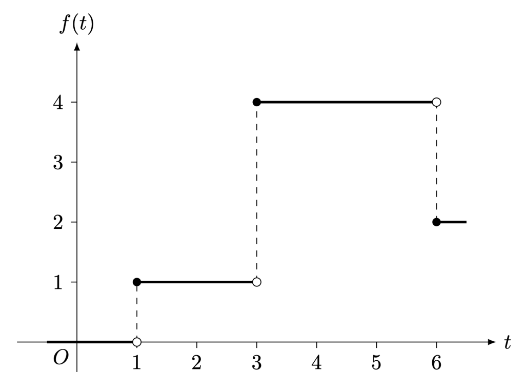
Question 2. The function $f$ is defined by the graph below.

Evaluate $\mathcal L\{(f(t))^2\}$ and $\mathcal L\{(f(t))^2 \cdot U(t-4)\}$ .

(Click for Solution)

Solution. By observation,

$f(t) = \begin{cases}0, &t < 1, \\ 1, & 1 \leq t < 3, \\ 4, & 3 \leq t < 6, \\ 2, & t \geq 6.\end{cases}$

By the definition of $f$ ,

$\begin{aligned} (f(t))^2 &= \begin{cases}0^2, &t < 1, \\ 1^2, & 1 \leq t < 3, \\ 4^2, & 3 \leq t < 6, \\ 2^2, & t \geq 6,\end{cases} = \begin{cases}0, &t < 1, \\ 1, & 1 \leq t < 3, \\ 16, & 3 \leq t < 6, \\ 4, & t \geq 6.\end{cases} \end{aligned}$

By the jump technique,

$\begin{aligned}(f(t))^2 &= 0 + (1-0)U(t-1) + (16-1)U(t-3) + (4-16)U(t-6) \\ &= U(t-1) + 15U(t-3) -12U(t-6). \end{aligned}$

By the linearity of Laplace transforms,

$\begin{aligned}\mathcal L\{ (f(t))^2 \} &= \mathcal L\{ U(t-1) \} + 15 \cdot \mathcal L\{ U(t-3) \} - 12 \cdot \mathcal L\{ U(t-6) \} \\ &= \frac{e^{-s}}{s} + 15 \cdot \frac{e^{-3s}}{s} - 12 \cdot \frac{e^{-6s}}{s} \\ &= \frac {1}s ( e^{-s} + 15e^{-3s} - 12 e^{-6s}). \end{aligned}$

Since $U(t-a) \cdot U(t-b) = U(t - \max\{a, b\})$ ,

$\begin{aligned} (f(t))^2 \cdot U(t-4) &= U(t-4) + 15U(t-4) -12U(t-6) \\ &= 16 U(t-4) -12 U(t-6). \end{aligned}$

Hence, by the linearity of Laplace transforms,

$\displaystyle \mathcal L\{(f(t))^2 \cdot U(t-4) \} = \frac 1s (16 e^{-4s} - 12 e^{-6s}).$

Question 3. Using the function $f$ defined in Question 2, evaluate

$\displaystyle \mathcal L\left\{\frac 1{1+f(t)} \cdot U(t-4) \right\}.$

(Click for Solution)

Solution. By the definition of $f$ ,

$\begin{aligned} \frac{1}{1+f(t)} &= \begin{cases} \frac{1}{1+0} , &t < 1, \\ \frac{1}{1+1}, & 1 \leq t < 3, \\ \frac{1}{1+4}, & 3 \leq t < 6, \\ \frac{1}{1+2}, & t \geq 6,\end{cases} = \begin{cases}1, &t < 1/2, \\ 1/2, & 1 \leq t < 3, \\ 1/5, & 3 \leq t < 6, \\ 1/3, & t \geq 6.\end{cases} \end{aligned}$

By the jump technique,

$\begin{aligned} \frac 1{1+f(t)} &= 1 + \left(\frac 12 - 1 \right) \cdot U(t-1) + \left(\frac 15 - \frac 12 \right) \cdot U(t-3) + \left(\frac 13 - \frac 15 \right) \cdot U(t-6) \\ &= 1 - \frac 12 \cdot U(t-1) - \frac 3{10} \cdot U(t-3) + \frac 2{15} \cdot U(t-6). \end{aligned}$

Since $U(t-a) \cdot U(t- 4) = U(t- \max \{a, 4\})$ ,

$\displaystyle \begin{aligned} \frac 1{1+f(t)} \cdot U(t-4) &= U(t- 4) - \frac 12 \cdot U(t- 4) - \frac 3{10} \cdot U(t- 4) + \frac 2{15} \cdot U(t-6) \\ &= \frac 1{5} \cdot U(t- 4) + \frac 2{15} \cdot U(t-6). \end{aligned}$

Taking Laplace transforms,

$\displaystyle \mathcal L \left\{ \frac 1{1+f(t)} \right\} = \frac 1s\left(\frac {e^{-4s}}{5} + \frac {2e^{-6s}}{15}\right).$

—Joel Kindiak, 18 Apr 25, 1558H

KindiakMath