So far, we have discussed numbers that:
- either have no direction, or
- have one dimension of direction.
We use positive numbers to represent either quantities with no direction, or quantities with some reasonable notion of “increase”. The larger the positive number, the larger the quantity.
Definition 1. For any positive number 

For the second case, we use negative numbers, namely numbers of the form 
- The quantity
Since 
Definition 2. For any real number

We also call 
- Note that we define
; indeed, the number
should denote some quantity with non-existent size.
Many a time, however, since we live in a three-dimensional world, it helps to have quantities that describe three-dimensional change. While what follows easily extends to three dimensions, we will keep discussions simple by working with just two dimensions.
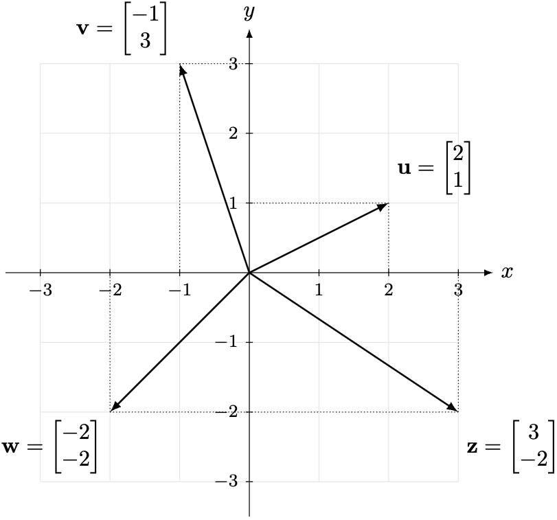
Definition 3. Define a two-dimensional vector by the object 

Using Pythagoras’ theorem, define the magnitude or the norm of the vector

Example 1. Using the diagram above,

We leave it as an exercise to verify that

Example 2. Let 
Solution. By Definition 3,

Now we consider two cases:
- If
, then
.
- If
, then
and
.
By Definition 2, 

Remark 1. Example 2 illustrates vectors as extensions of the numbers that we are familiar with (not without its limitations). Hence, we can describe
This characterisation of vectors turns out to be incredibly useful in making sense of two-dimensional quantities. However, we need to define meaningful calculations to actually use them.
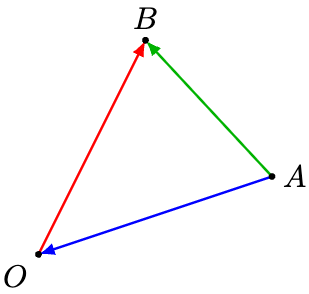
Consider the vectors 

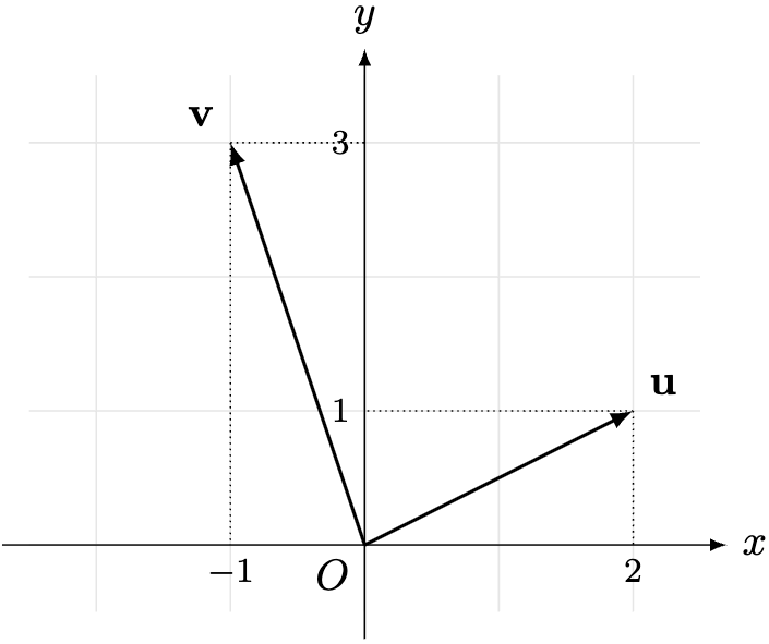
What do we mean by 


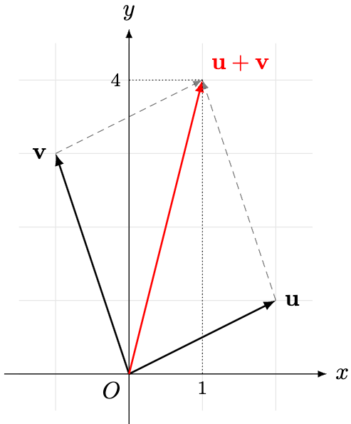
An equivalent interpretation is to create a parallelogram using

Therefore, we are justified in making the following definition for vector addition. We include scalar multiplication using similar intuitions.
Definition 4. Define vector addition and scalar multiplication as follows:

In particular, given the two-dimensional vectors 
, and
.
Example 3. Let 


Solution. Suppose 

By the definition of scalar multiplication,

Finally by the definition of vector subtraction and scalar multiplication,

For much more detail and insight, check out my fuller suite of posts on linear algebra here. Linear algebra, at its core, is the very first bridge between geometry and algebra that any student encounters.
Theorem 1. Consider the line 


In this case, we call the vector 

Proof Sketch. Define 

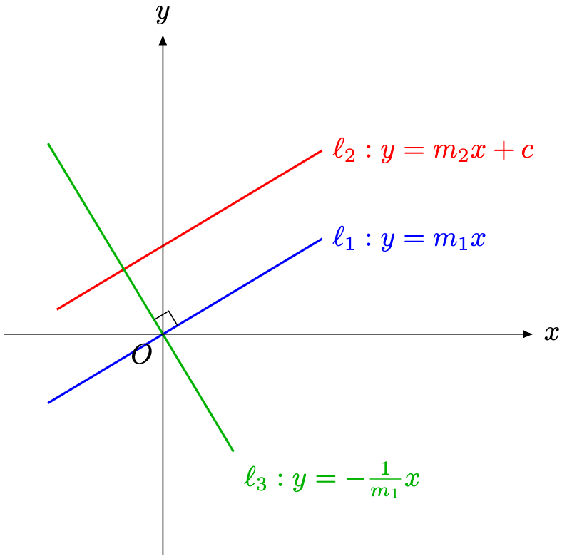
Theorem 2. Define the lines 


Proof Sketch. Consider the diagram below.
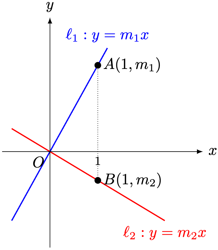
Using Pythagoras’ theorem,

Therefore, by Pythagoras’ theorem and its converse, 


We leave it as an exercise in algebra to simplify this equation to

Theorem 3. Define the lines 


Remark 2. Observe the deliberate omission of a diagram in Theorem 3. The power of vectors (i.e. linear algebra) is to describe geometry without a need for visual representation (though the latter will be useful for us in the process of proving the result).
Proof Sketch. Define the line 


Since the interior angles of a pair of lines sum to 

Corollary 1. Consider the lines

where
Proof. Define 


Theorem 4. Let 


where we abbreviate 


Proof Sketch. Use Theorems 1 and 3.
There are many more implications of thinking in terms of vectors, but we conclude with the famous intercept theorem.
Lemma 1. Given two points 


Then 
Proof. Using vector addition,

Theorem 5 (Intercept Theorem). Given three distinct points 


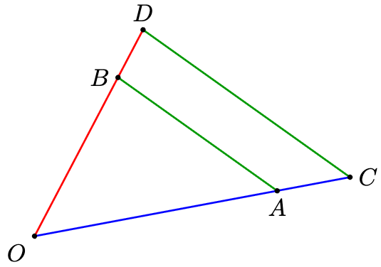
(Here, we assume 
Then 


Proof Sketch. Denote 


In the direction 


By Theorem 4,
In the direction 

Now 


In a similar manner with the other sides,

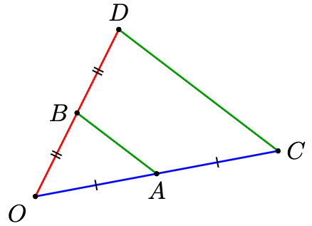
Corollary 2 (Midpoint Theorem). If we have

then 
Proof. By hypothesis, set 
In this case, we call 

Using this idea of describing shapes using coordinates, we turn to parabolas, and namely, analyse graphs of the form 
—Joel Kindiak, 22 Oct 25, 2217H

Leave a comment