Integrating rational functions can get quite challenging unless we split it up into a sum of “smaller” rational functions whose integrals are relatively more trivial to compute.
Questions
Question 1. Evaluate the integral .
(Click for Solution)
Solution. Factorise , so that
Using the cover-up rule to make the following calculations:
For , set so that .
For , set so that .
For , set so that .
In particular, and , so that
AlternateSolution. We observe that
Making the substitution , we decompose
Using the cover-up rule,
Therefore,
Finally, we make the clever observation that
so that
Therefore,
Question 2. Evaluate the integral .
(Click for Solution)
Solution. First make the clever factorisation
Then use the partial fraction decomposition
Now the roots of are . Therefore, using in the cover-up rule,
Likewise, the roots of are . Therefore, using in the cover-up rule,
Problem 3. Use Problem 2 to prove Young’s inequality: for any ,
with equality if and only if .
(Click for Solution)
Solution. Setting ,
Furthermore, since , equality holds if and only if
Problem 4. Use Young’s inequality to prove Hölder’s inequality for two-dimensional vectors: given non-negative numbers ,
(Click for Solution)
Solution. If , then implies , and the inequality holds trivially. Without loss of generality, suppose the right-hand side is non-zero. It suffices to prove that
By one application of Young’s inequality,
By a second application of Young’s inequality,
Summing the inequalities,
Problem 5. Use Hölder’s inequality to prove Minkowski’s inequality for two-dimensional vectors: given real numbers ,
(Click for Solution)
Solution. By the vanilla triangle inequality,
By Hölder’s inequality,
so that
Similarly,
Combining the displays,
The result follows by the observation
Remark 1. Denoting
and defining , Hölder’s inequality reduces to
and Minkowski’s inequality reduces to
Setting reduces to the usual Cauchy-Schwarz inequality and triangle inequality for two-dimensional vectors. Furthermore, these results hold for -dimensional vectors, and even “infinite-dimensional” (sufficiently nice) functions.
We regard integration, at the pre-university level, as the reverse process of differentiation:
We call the integrand. Integration is linear in the following sense:
The integrals of powers requires a bit more care: if then nothing weird happens:
However, if , then we cannot divide by zero, and instead recover the logarithm:
Other commonly used integrals are free for use. Furthermore, in the context of pre-university mathematics, the definite integral is an application of the vanilla integral:
Questions
You may not use integration by substitution in any of these problems.
Question 1. Evaluate .
(Click for Solution)
Solution. Simplifying the integrand then integrating term-wise,
Question 2. Evaluate .
(Click for Solution)
Solution. We first slowly expand the integrand:
Using linearity to integrate term-wise,
Question 3. Evaluate .
(Click for Solution)
Solution. We first slowly expand the integrand:
Using linearity to integrate term-wise,
Remark 1. In general, when feasible, final answers ought to take the form
where are numerical constants, are expressions in terms of , and denotes the arbitrary constant of integration (if and only if needed), for easy recognition.
To maximise (or minimise) a quantity , we apply the zero derivative condition
and check that the corresponding value yields to a maximum (resp. minimum) via the second derivative test:
a local maximum is obtained at when ,
a local minimum is obtained at when .
Recall that we denote
for brevity.
Questions
Question 1. Evaluate the area of the largest rectangle contained inside the ellipse graphed below.
(Click for Solution)
Solution. Given , the base of the rectangle is and its height is , yielding a total area of . Differentiating with respect to ,
On the other hand, given the ellipse , differentiate with respect to on both sides to obtain
Therefore,
By the zero-derivative condition, if is maximised, then :
Plugging back into the equation of the ellipse,
since , yielding . Thus, the area of the corresponding rectangle is .
To apply second derivative test, we differentiate again:
so is indeed maximised when and .
Question 2. The diagram below shows a movie theatre with a screen tall, whose base is above the ground.
The permissible viewing area is long with an incline of up to . Determine the position that a movie-goer should sit in order to maximise his viewing angle , justifying your answer.
(Click for Solution)
Solution. Let denote the horizontal distance of the movie-goer from the screen. His height is then determined using similar triangles:
By observation,
We remark that if , then and the formula still works. Differentiating with respect to ,
By the zero-derivative condition, if is maximised, then :
We need to (painfully) solve this equation:
since .
To apply second derivative test, we differentiate again:
When , , so that
so indeed will attain its maximum at .
Question 3. Determine the smallest perimeter of a rectangle with area .
(Click for Solution)
Solution. Let denote the base and height of the rectangle respectively. Since implies , the perimeter of the rectangle is given by
Differentiating twice,
Solving yields so that . Since automatically, yields a (local) minimum for . Hence, the rectangle has a minimum perimeter of , which corresponds to the rectangle being a square with base length .
Remark 1. The result remains true even if we consider rectangles of other areas; the rectangle with area whose perimeter is minimum must be a square with side length .
Question 4. Given that , maximise .
(Click for Solution)
Solution. Define . Differentiating twice,
Solving , since , . Substituting into ,
so that yields a local (global) maximum. Hence, has a maximum value of
Remark 2. Using the same technique, we can prove that for any and ,
with equality at . Setting yields Question 4.
Question 5. Given that , find the value of that minimises .
(Click for Solution)
Solution. Define . Differentiating twice,
Therefore, is minimised when :
since .
Remark 3. In general, the value of that minimises is given by .
Question 2. A man of height metres is currently away from a pole of height . He runs in a straight line towards the pole at a speed of . Let denote the angle of elevation from the man to the top of the pole.
Evaluate the rate of change of when the man is at the pole.
(Click for Solution)
Solution. The man’s distance from the pole at time is given by metres. By considering the height difference between the pole and the man,

![[a, b]](https://s0.wp.com/latex.php?latex=%5Ba%2C+b%5D&bg=ffffff&fg=000&s=0&c=20201002)


![[a,b] = [0,1]](https://s0.wp.com/latex.php?latex=%5Ba%2Cb%5D+%3D+%5B0%2C1%5D&bg=ffffff&fg=000&s=0&c=20201002)


![\displaystyle \lim_{n \to \infty} \frac{\sqrt[3]{1} + \sqrt[3]{2} + \cdots + \sqrt[3]{n}}{n\sqrt[3]{n}}](https://s0.wp.com/latex.php?latex=%5Cdisplaystyle+%5Clim_%7Bn+%5Cto+%5Cinfty%7D+%5Cfrac%7B%5Csqrt%5B3%5D%7B1%7D+%2B+%5Csqrt%5B3%5D%7B2%7D+%2B+%5Ccdots+%2B+%5Csqrt%5B3%5D%7Bn%7D%7D%7Bn%5Csqrt%5B3%5D%7Bn%7D%7D&bg=ffffff&fg=000&s=0&c=20201002)


![\begin{aligned} \lim_{n \to \infty} \frac{\sqrt[3]{1} + \sqrt[3]{2} + \cdots + \sqrt[3]{n}}{n\sqrt[3]{n}} &= \lim_{n \to \infty} \sum_{k=1}^n \frac{\sqrt[3]{k}}{n\sqrt[3]{n}} = \lim_{n \to \infty} \sum_{k=1}^n \sqrt[3]{\frac kn } \cdot \frac 1n \\ &= \lim_{n \to \infty} \sum_{k=1}^n \sqrt[3]{x_k} \cdot \Delta x_k = \int_0^1 \sqrt[3]{x}\, \mathrm dx \\ &= \int_0^1 x^{1/3}\, \mathrm dx = \left[ \frac{x^{4/3}}{4/3} \right]_0^1 = \frac 34. \end{aligned}](https://s0.wp.com/latex.php?latex=%5Cbegin%7Baligned%7D+%5Clim_%7Bn+%5Cto+%5Cinfty%7D+%5Cfrac%7B%5Csqrt%5B3%5D%7B1%7D+%2B+%5Csqrt%5B3%5D%7B2%7D+%2B+%5Ccdots+%2B+%5Csqrt%5B3%5D%7Bn%7D%7D%7Bn%5Csqrt%5B3%5D%7Bn%7D%7D+%26%3D+%5Clim_%7Bn+%5Cto+%5Cinfty%7D+%5Csum_%7Bk%3D1%7D%5En+%5Cfrac%7B%5Csqrt%5B3%5D%7Bk%7D%7D%7Bn%5Csqrt%5B3%5D%7Bn%7D%7D+%3D+%5Clim_%7Bn+%5Cto+%5Cinfty%7D+%5Csum_%7Bk%3D1%7D%5En+%5Csqrt%5B3%5D%7B%5Cfrac+kn+%7D+%5Ccdot+%5Cfrac+1n+%5C%5C+%26%3D+%5Clim_%7Bn+%5Cto+%5Cinfty%7D+%5Csum_%7Bk%3D1%7D%5En+%5Csqrt%5B3%5D%7Bx_k%7D+%5Ccdot+%5CDelta+x_k+%3D+%5Cint_0%5E1+%5Csqrt%5B3%5D%7Bx%7D%5C%2C+%5Cmathrm+dx+%5C%5C+%26%3D+%5Cint_0%5E1+x%5E%7B1%2F3%7D%5C%2C+%5Cmathrm+dx+%3D+%5Cleft%5B+%5Cfrac%7Bx%5E%7B4%2F3%7D%7D%7B4%2F3%7D+%5Cright%5D_0%5E1+%3D+%5Cfrac+34.+%5Cend%7Baligned%7D&bg=ffffff&fg=000&s=0&c=20201002)
 .
. , so that
 , set
, set  so that
  .
. , set
, set  .
. , set
, set  so that
  .
. and
and  , so that

 , we decompose


 .
.

 are
are  . Therefore, using
  in the cover-up rule,
 are
are  . Therefore, using
  in the cover-up rule,


 is taken from the easier-to-integrate function
  .
. , define
 and
and  . Hence, evaluate
  in terms of
 ![\begin{aligned} I_0 &= \int_0^{\pi} \sin^0(x)\, \mathrm dx = \int_0^{\pi}\, \mathrm dx = \pi, \\ I_1 &= \int_0^{\pi} \sin(x)\, \mathrm dx = \left[ - \cos(x) \right]_0^{\pi} \\ &= (-(-1) - (-1)) = 2. \end{aligned}](https://s0.wp.com/latex.php?latex=%5Cbegin%7Baligned%7D+I_0+%26%3D+%5Cint_0%5E%7B%5Cpi%7D+%5Csin%5E0%28x%29%5C%2C+%5Cmathrm+dx+%3D+%5Cint_0%5E%7B%5Cpi%7D%5C%2C+%5Cmathrm+dx+%3D+%5Cpi%2C+%5C%5C+I_1+%26%3D+%5Cint_0%5E%7B%5Cpi%7D+%5Csin%28x%29%5C%2C+%5Cmathrm+dx+%3D+%5Cleft%5B+-+%5Ccos%28x%29+%5Cright%5D_0%5E%7B%5Cpi%7D+%5C%5C+%26%3D+%28-%28-1%29+-+%28-1%29%29+%3D+2.+%5Cend%7Baligned%7D&bg=ffffff&fg=000&s=0&c=20201002)
 , so that
![\begin{aligned} &\int_0^{\pi} \sin^{n-2}(x) \cos^2(x) \, \mathrm dx \\ &= \int_0^{\pi} \sin^{n-2}(x) \cos(x) \cdot \cos(x) \, \mathrm dx \\ &= \left[ \underbrace{ \phantom- \frac{\sin^{n-1}(x)}{n-1} \phantom- }_{\mathrm I}\, \underbrace{ \phantom- \cos(x) \phantom- }_{\mathrm S} \right]_0^{\pi} - \int_0^{\pi} \underbrace{ \phantom- \frac{\sin^{n-1}(x)}{n-1} \phantom- }_{\mathrm I}\, \underbrace{ \phantom- (-\sin(x))\, \mathrm dx \phantom- }_{\mathrm D} \\ &= (0 - 0) + \frac 1{n-1} \int_0^{\pi} \sin^n(x)\, \mathrm dx = \frac 1{n-1} \cdot I_{n}. \end{aligned}](https://s0.wp.com/latex.php?latex=%5Cbegin%7Baligned%7D+%26%5Cint_0%5E%7B%5Cpi%7D+%5Csin%5E%7Bn-2%7D%28x%29+%5Ccos%5E2%28x%29+%5C%2C+%5Cmathrm+dx+%5C%5C+%26%3D+%5Cint_0%5E%7B%5Cpi%7D+%5Csin%5E%7Bn-2%7D%28x%29+%5Ccos%28x%29+%5Ccdot+%5Ccos%28x%29+%5C%2C+%5Cmathrm+dx+%5C%5C+%26%3D+%5Cleft%5B+%5Cunderbrace%7B+%5Cphantom-+%5Cfrac%7B%5Csin%5E%7Bn-1%7D%28x%29%7D%7Bn-1%7D+%5Cphantom-+%7D_%7B%5Cmathrm+I%7D%5C%2C+%5Cunderbrace%7B+%5Cphantom-+%5Ccos%28x%29+%5Cphantom-+%7D_%7B%5Cmathrm+S%7D+%5Cright%5D_0%5E%7B%5Cpi%7D+-+%5Cint_0%5E%7B%5Cpi%7D+%5Cunderbrace%7B+%5Cphantom-+%5Cfrac%7B%5Csin%5E%7Bn-1%7D%28x%29%7D%7Bn-1%7D+%5Cphantom-+%7D_%7B%5Cmathrm+I%7D%5C%2C+%5Cunderbrace%7B+%5Cphantom-+%28-%5Csin%28x%29%29%5C%2C+%5Cmathrm+dx+%5Cphantom-+%7D_%7B%5Cmathrm+D%7D+%5C%5C+%26%3D+%280+-+0%29+%2B+%5Cfrac+1%7Bn-1%7D+%5Cint_0%5E%7B%5Cpi%7D+%5Csin%5En%28x%29%5C%2C+%5Cmathrm+dx+%3D+%5Cfrac+1%7Bn-1%7D+%5Ccdot+I_%7Bn%7D.+%5Cend%7Baligned%7D&bg=ffffff&fg=000&s=0&c=20201002)


 where
where  ,
,
 if
if  and
and  if
if  .
.
 . Finally, evaluate
  .
. ,
,![\begin{aligned} I_0 &= \int_{-1}^{1} \frac 1{\sqrt{2x+3}}\, \mathrm dx = \int_{-1}^{1} (2x+3)^{-1/2}\, \mathrm dx \\ &= \left[ \frac 12 \cdot \frac{(2x+3)^{1/2}}{1/2} \right]_{-1}^1 = \left[ \sqrt{2x+3} \right]_{-1}^1 = -1 + \sqrt 5. \end{aligned}](https://s0.wp.com/latex.php?latex=%5Cbegin%7Baligned%7D+I_0+%26%3D+%5Cint_%7B-1%7D%5E%7B1%7D+%5Cfrac+1%7B%5Csqrt%7B2x%2B3%7D%7D%5C%2C+%5Cmathrm+dx+%3D+%5Cint_%7B-1%7D%5E%7B1%7D+%282x%2B3%29%5E%7B-1%2F2%7D%5C%2C+%5Cmathrm+dx+%5C%5C+%26%3D+%5Cleft%5B+%5Cfrac+12+%5Ccdot+%5Cfrac%7B%282x%2B3%29%5E%7B1%2F2%7D%7D%7B1%2F2%7D+%5Cright%5D_%7B-1%7D%5E1+%3D+%5Cleft%5B+%5Csqrt%7B2x%2B3%7D+%5Cright%5D_%7B-1%7D%5E1+%3D+-1+%2B+%5Csqrt+5.+%5Cend%7Baligned%7D&bg=ffffff&fg=000&s=0&c=20201002)
 ,
,![\begin{aligned} I_n &= \int_{-1}^1 \frac{ x^n }{ \sqrt{2x+3} }\, \mathrm dx \\ &= \int_{-1}^1 x^n \cdot \frac{ 1 }{ \sqrt{2x+3} }\, \mathrm dx \\ &= \frac 12 \int_{-1}^1 x^{n-1} \cdot \frac{ (2x+3-3) }{ \sqrt{2x+3} }\, \mathrm dx \\ &= \frac 12 \int_{-1}^1 x^{n-1} \sqrt{2x+3}\, \mathrm dx - \frac 32 \int_{-1}^1 x^{n-1} \cdot \frac 1{\sqrt{2x+3}}\, \mathrm dx \\ &= \frac 12 \left( \left[\underbrace{ \phantom- \frac{x^n}{n} \phantom- }_{\mathrm I}\cdot \underbrace{ \phantom- \sqrt{2x+3} \phantom- }_{\mathrm S} \right]_{-1}^1 - \int_{-1}^1 \underbrace{ \phantom- \frac{x^n}{n} \phantom- }_{\mathrm I}\cdot \underbrace{ \phantom- \frac{1}{2\sqrt{2x+3}} \cdot 2 \, \mathrm dx\phantom- }_{\mathrm D}\right) - \frac 32 \cdot I_{n-1} \\ &= \frac 12 \left( \frac 1n \cdot (\sqrt 5 - (-1)^n) - \frac 1n \cdot I_n \right) - \frac 32 \cdot I_{n-1} \\ &=\frac 1{2n} \cdot (\sqrt 5 - (-1)^n) - \frac 1{2n} \cdot I_n - \frac 32 \cdot I_{n-1}. \end{aligned}](https://s0.wp.com/latex.php?latex=%5Cbegin%7Baligned%7D+I_n+%26%3D+%5Cint_%7B-1%7D%5E1+%5Cfrac%7B+x%5En+%7D%7B+%5Csqrt%7B2x%2B3%7D+%7D%5C%2C+%5Cmathrm+dx+%5C%5C+%26%3D+%5Cint_%7B-1%7D%5E1+x%5En+%5Ccdot+%5Cfrac%7B+1+%7D%7B+%5Csqrt%7B2x%2B3%7D+%7D%5C%2C+%5Cmathrm+dx+%5C%5C+%26%3D+%5Cfrac+12+%5Cint_%7B-1%7D%5E1+x%5E%7Bn-1%7D+%5Ccdot+%5Cfrac%7B+%282x%2B3-3%29+%7D%7B+%5Csqrt%7B2x%2B3%7D+%7D%5C%2C+%5Cmathrm+dx+%5C%5C+%26%3D+%5Cfrac+12+%5Cint_%7B-1%7D%5E1+x%5E%7Bn-1%7D+%5Csqrt%7B2x%2B3%7D%5C%2C+%5Cmathrm+dx+-+%5Cfrac+32+%5Cint_%7B-1%7D%5E1+x%5E%7Bn-1%7D+%5Ccdot+%5Cfrac+1%7B%5Csqrt%7B2x%2B3%7D%7D%5C%2C+%5Cmathrm+dx+%5C%5C+%26%3D+%5Cfrac+12+%5Cleft%28+%5Cleft%5B%5Cunderbrace%7B+%5Cphantom-+%5Cfrac%7Bx%5En%7D%7Bn%7D+%5Cphantom-+%7D_%7B%5Cmathrm+I%7D%5Ccdot+%5Cunderbrace%7B+%5Cphantom-+%5Csqrt%7B2x%2B3%7D+%5Cphantom-+%7D_%7B%5Cmathrm+S%7D+%5Cright%5D_%7B-1%7D%5E1+-+%5Cint_%7B-1%7D%5E1+%5Cunderbrace%7B+%5Cphantom-+%5Cfrac%7Bx%5En%7D%7Bn%7D+%5Cphantom-+%7D_%7B%5Cmathrm+I%7D%5Ccdot+%5Cunderbrace%7B+%5Cphantom-+%5Cfrac%7B1%7D%7B2%5Csqrt%7B2x%2B3%7D%7D+%5Ccdot+2++%5C%2C+%5Cmathrm+dx%5Cphantom-+%7D_%7B%5Cmathrm+D%7D%5Cright%29+-+%5Cfrac+32+%5Ccdot+I_%7Bn-1%7D+%5C%5C+%26%3D+%5Cfrac+12+%5Cleft%28+%5Cfrac+1n+%5Ccdot+%28%5Csqrt+5+-+%28-1%29%5En%29+-+%5Cfrac+1n+%5Ccdot+I_n+%5Cright%29+-+%5Cfrac+32+%5Ccdot+I_%7Bn-1%7D+%5C%5C+%26%3D%5Cfrac+1%7B2n%7D+%5Ccdot+%28%5Csqrt+5+-+%28-1%29%5En%29+-+%5Cfrac+1%7B2n%7D+%5Ccdot+I_n++-+%5Cfrac+32+%5Ccdot+I_%7Bn-1%7D.+%5Cend%7Baligned%7D&bg=ffffff&fg=000&s=0&c=20201002)


 such that
  .
. .
.
 ,
,  with equality if and only if
  . By observation,

 yields a global minimum:
 for any
  ,
,
 .
. ,
,
 , equality holds if and only if
 ,
,
 , then
  implies
  , and the inequality holds trivially. Without loss of generality, suppose the right-hand side is non-zero. It suffices to prove that


 , Hölder’s inequality reduces to

 reduces to the usual Cauchy-Schwarz inequality and
  allows us to simplify integrals:

 , evaluate the integral
  .
. .
. ,
,
![\begin{aligned} \int_0^1 xe^{-x^2}\, \mathrm dx &= \left[ -\frac 12 \cdot e^{-x^2} \right]_0^1 \\ &= \left( -\frac 12 \cdot e^{-1^2} \right) - \left( -\frac 12 \cdot e^{-0^2} \right) \\ &= \frac 12(1-e^{-1}). \end{aligned}](https://s0.wp.com/latex.php?latex=%5Cbegin%7Baligned%7D+%5Cint_0%5E1+xe%5E%7B-x%5E2%7D%5C%2C+%5Cmathrm+dx+%26%3D+%5Cleft%5B+-%5Cfrac+12+%5Ccdot+e%5E%7B-x%5E2%7D++%5Cright%5D_0%5E1+%5C%5C+%26%3D+%5Cleft%28+-%5Cfrac+12+%5Ccdot+e%5E%7B-1%5E2%7D+%5Cright%29+-+%5Cleft%28+-%5Cfrac+12+%5Ccdot+e%5E%7B-0%5E2%7D+%5Cright%29+%5C%5C+%26%3D+%5Cfrac+12%281-e%5E%7B-1%7D%29.+%5Cend%7Baligned%7D&bg=ffffff&fg=000&s=0&c=20201002)


 .
. ,
,
 so that
 ,
,

 the integrand. Integration is linear in the following sense:
 then nothing weird happens:
 , then we cannot divide by zero, and instead recover the logarithm:
![\displaystyle \int_a^b f(x)\, \mathrm dx := F(b) - F(a) \equiv [F(x)]_a^b.](https://s0.wp.com/latex.php?latex=%5Cdisplaystyle+%5Cint_a%5Eb+f%28x%29%5C%2C+%5Cmathrm+dx+%3A%3D+F%28b%29+-+F%28a%29+%5Cequiv+%5BF%28x%29%5D_a%5Eb.&bg=ffffff&fg=000&s=0&c=20201002)
 .
.
 .
.

 .
.


 are numerical constants,
  are expressions in terms of
  , and
, and  denotes the arbitrary constant of integration (if and only if needed), for easy recognition.
 , we apply the zero derivative condition
 yields to a maximum (resp. minimum) via the second derivative test:
 when
when  ,
, .
.
 , the base of the rectangle is
  and its height is
  , yielding a total area of
  . Differentiating with respect to
 , differentiate with respect to

 :
:

 , yielding
  . Thus, the area of the corresponding rectangle is
  .
.
 and
and  .
. tall, whose base is
  above the ground.
 long with an incline of up to
  . Determine the position that a movie-goer
  should sit in order to maximise his viewing angle
  , justifying your answer.

 , then
  and the formula still works. Differentiating with respect to
 :
:


 ,
,  , so that
 .
. .
. denote the base and height of the rectangle respectively. Since
  implies
  , the perimeter

 yields
  . Since
  automatically,
  , which corresponds to the rectangle being a square with base length
  .
. , maximise
  .
. . Differentiating twice,
 . Substituting into
  ,
,
 yields a local (global) maximum. Hence,
 and
and  ,
,
 . Setting
  yields Question 4.
 .
. . Differentiating twice,
![\displaystyle 18x^2 - 35x^{-6} = 0 \quad \Rightarrow \quad x^8 = \frac{35}{18} \quad \Rightarrow \quad x = \sqrt[8]{ \frac{ 35 }{ 18 } },](https://s0.wp.com/latex.php?latex=%5Cdisplaystyle+18x%5E2+-+35x%5E%7B-6%7D+%3D+0+%5Cquad+%5CRightarrow+%5Cquad+x%5E8+%3D+%5Cfrac%7B35%7D%7B18%7D+%5Cquad+%5CRightarrow+%5Cquad+x+%3D+%5Csqrt%5B8%5D%7B+%5Cfrac%7B+35+%7D%7B+18+%7D+%7D%2C&bg=ffffff&fg=000&s=0&c=20201002)
 is given by
  .
. in terms of time
  is
is  . Furthermore, given
  , the chain rule yields
 above the
 . Let
. Let  denote the intersection of
  with the
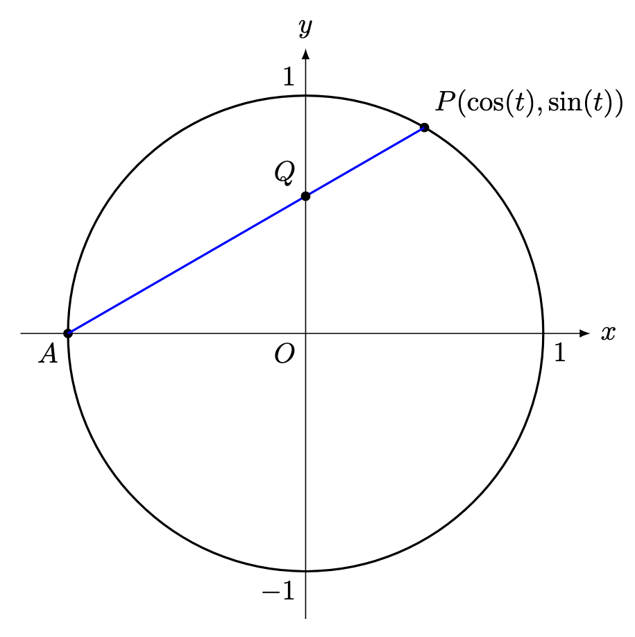
 .
.

 denote the
 , so that

 , since
  ,
,


 metres is currently
  away from a pole of height
  . He runs in a straight line towards the pole at a speed of
  . Let
. Let 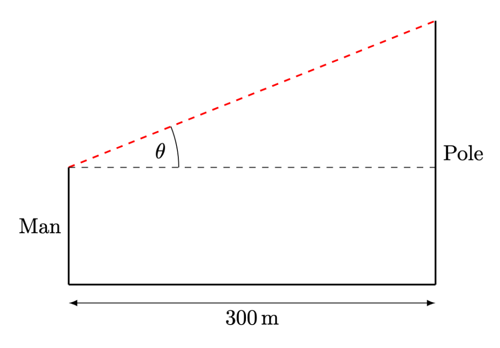
 metres. By considering the height difference between the pole and the man,

 , so that


 , then
 .
.


 .
. , applying the chain rule repeatedly and carefully,
 .
.
 , denoted
  , intuitively measures the gradient of the tangent to
  at
at  . For any general


 .
.
 .
.
 .
.

 .
.

