Category: Calculus

Tricky Limits

Big Idea

We write $\displaystyle \lim_{x \to c} f(x) = L$ to mean that $f(x) \to L$ as $x \to c$ . In particular, if $g$ is continuous at $c$ and $f(x) = g(x)$ for $x \neq c$ , then

$\displaystyle \lim_{x \to c} f(x) = \lim_{x \to c} g(x) = g(c).$

Furthermore, the usual limit laws hold.

Questions

Question 1. Evaluate the limit $\displaystyle \lim_{x \to 2} \frac{x^2 - 4}{x^3 - 8}$ .

(Click for Solution)

Solution. Since $2$ is a root of $x^3 - 8$ , $x-2$ is a factor of $x^3 - 8$ :

$\begin{aligned} x^3 - 8 &= (x-2)(x^2 + kx + 4) \\ &= x^3 + (k-2)x^2 +(4-2k)x - 8. \end{aligned}$

Comparing coefficients, $k = 2$ . Hence,

$\begin{aligned} \lim_{x \to 2} \frac{x^2 - 4}{x^3 - 8} &= \lim_{x \to 2} \frac{(x-2)(x+2)}{(x-2)(x^2 + 2x + 4)} \\ &= \lim_{x \to 2} \frac{x+2}{x^2 + 2x + 4} \\ &= \frac{2+2}{2^2 + 2\cdot 2 + 4} = \frac 13.\end{aligned}$

Alternate Solution. Make the substitution $x = 2 +t$ , so that $x \to 2$ leads to $t \to 2$ . Then

$\begin{aligned} \lim_{x \to 2} \frac{x^2 - 4}{x^3 - 8} &= \lim_{t \to 0} \frac{(2+t)^2 - 4}{(2+t)^3 - 8} \\ &= \lim_{t \to 0} \frac{ (4 + 4t + t^2) - 4}{ (8 + 12t + 6t + t^3) - 8} \\ &= \lim_{t \to 0} \frac{ 4t + t^2 }{ 12t + 6t^2 + t^3 } \\ &= \lim_{t \to 0} \frac{ 4 + t }{ 12 + 6t + t^2 } \\ &= \frac{ 4 + 0 }{ 12 + 6 \cdot 0 + 0^2 } = \frac 13.\end{aligned}$

Question 2. Evaluate the limit $\displaystyle \lim_{x \to 4} \frac{\sqrt{1+2x} - 3}{\sqrt x-2}$ .

(Click for Solution)

Solution. Rationalising both numerator and denominator,

$\begin{aligned} \lim_{x \to 4} \frac{\sqrt{1+2x} - 3}{\sqrt x-2} &= \lim_{x \to 4} \left( (\sqrt{1+2x} - 3) \cdot \frac{1}{\sqrt x-2} \right) \\ &= \lim_{x \to 4} \left( (\sqrt{1+2x} - 3) \cdot \frac{\sqrt{1+2x} + 3}{\sqrt{1+2x} + 3} \cdot \frac{1}{\sqrt x-2} \cdot \frac{\sqrt x + 2}{\sqrt x + 2} \right) \\ &= \lim_{x \to 4} \left( \frac{(1+2x) - 9}{\sqrt{1+2x} + 3} \cdot \frac{\sqrt x + 2}{x-4} \right) \\ &= \lim_{x \to 4} \left( \frac{ 2(x-4) }{\sqrt{1+2x} + 3} \cdot \frac{\sqrt x + 2}{x-4} \right) \\ &= 2\cdot \lim_{x \to 4} \frac{ \sqrt x + 2 }{\sqrt{1+2x} + 3} = 2 \cdot \frac{\sqrt 4+2}{\sqrt{1 + 2 \cdot 4} + 3} = \frac 43. \end{aligned}$

Question 3. Evaluate the limit $\displaystyle \lim_{x \to \infty} \frac{\sqrt{4x^2 + 5}}{\sqrt[3]{x^3 - 1}}$ .

(Click for Solution)

Solution. By factoring $x = \sqrt{x^2} = \sqrt[3]{x^3}$ on both the numerator and the denominator,

$\begin{aligned} \lim_{x \to \infty} \frac{\sqrt{4x^2 + 5}}{\sqrt[3]{x^3 - 1}} &= \lim_{x \to \infty} \frac{\sqrt{x^2 \cdot (4 + 5 / x^2)}}{\sqrt[3]{x^3 \cdot (1 - 1/ x^3)}} \\ &= \lim_{x \to \infty} \frac{\sqrt{x^2} \cdot \sqrt{ 4 + 5 / x^2 }}{\sqrt[3]{x^3} \cdot \sqrt[3]{ 1 - 1/x^3 } } \\ &= \lim_{x \to \infty} \frac{x \cdot \sqrt{ 4 + 5/ x^{2} }}{x \cdot \sqrt[3]{ 1 - 1/x^{3} } } \\&= \lim_{x \to \infty} \frac{\sqrt{ 4 + 5 /x^{2} }}{\sqrt[3]{ 1 - 1/x^{3} } } = \frac{\sqrt{ 4 + 0 }}{\sqrt[3]{ 1 - 0 } } = 2. \end{aligned}$

—Joel Kindiak, 3 Sept 25, 1804H

October 23, 2025
Some Normal Distribution Trivia
Problem 1. Let $f$ be a continuously differentiable function. Evaluate $\displaystyle \int x f'(x^2)\, \mathrm dx$ . Hence, evaluate

$\displaystyle \int x e^{-x^2}\, \mathrm dx,\quad \int \frac{x}{1+x^4}\, \mathrm dx.$

(Click for Solution)

Solution. Make the substitution $u = x^2 \Rightarrow \frac 12 \mathrm du = x\, \mathrm dx$ so that

$\begin{aligned} \int x f'(x^2)\, \mathrm dx &= \int f'(u) \cdot \frac 1{2}\, \mathrm du \\ &= \frac 12 \int f'(u)\, \mathrm du \\ &= \frac 12 f(u) + C \\ &= \frac 12 f(x^2) + C. \end{aligned}$

Particularise the result to $f(x) = -e^{-x}$ and $f(x) = \tan^{-1}(x)$ to obtain

$\displaystyle \int x e^{-x^2}\, \mathrm dx = -\frac 12 e^{-x^2} + C,\quad \int \frac{x}{1+x^4}\, \mathrm dx = \frac 12 \tan^{-1}(x) + C.$

Assume the following integral identity

$\displaystyle \left( \int_{-\infty}^{\infty} e^{-x^2}\, \mathrm dx \right)^2 = \int_0^{\infty} 2 \pi x e^{-x^2}\, \mathrm dx.$

Problem 2. Evaluate $\displaystyle \int_{-\infty}^{\infty} x^n e^{-x^2}\, \mathrm dx$ for $n = 0, 1, 2$ .

(Click for Solution)

Solution. For $n = 0$ , we use the given identity

$\begin{aligned} \left( \int_{-\infty}^{\infty} e^{-x^2}\, \mathrm dx \right)^2 &= \int_0^{\infty} 2 \pi x e^{-x^2}\, \mathrm dx \\ &= 2\pi \int_0^{\infty} xe^{-x^2}\, \mathrm dx \\ &= 2\pi \left[-\frac 12 e^{-x^2}\right]_0^\infty \\ &= 2\pi \left(-\frac 12 \cdot 0 + \frac 12 \cdot 1\right) = \pi. \end{aligned}$

Hence, $\displaystyle \int_{-\infty}^{\infty} e^{-x^2}\, \mathrm dx = \sqrt{\pi}$ . For $n = 1$ ,

$\begin{aligned}\int_0^{\infty} x e^{-x^2}\, \mathrm dx &= \left[-\frac 12 e^{-x^2}\right]_{-\infty}^\infty = -\frac 12 \cdot 0 + \frac 12 \cdot 0 = 0. \end{aligned}$

For $n = 2$ , we first integrate by parts to get

$\begin{aligned} \int x^2 e^{-x^2}\, \mathrm dx &= \int x \cdot x e^{-x^2}\, \mathrm dx \\ &= \underbrace{ -\frac 12 e^{-x^2} }_{\mathrm I} \underbrace{ x }_{\mathrm S} - \int \underbrace{ -\frac 12 e^{-x^2} }_{\mathrm I} \underbrace{ 1 }_{\mathrm D}\, \mathrm dx \\ &= -\frac 12 xe^{-x^2} + \frac 12 \int e^{-x^2}\, \mathrm dx. \end{aligned}$

Plugging in the limits,

$\displaystyle \begin{aligned} \int_{-\infty}^{\infty} x^2 e^{-x^2}\, \mathrm dx &= \left[ -\frac 12 xe^{-x^2} \right]_{-\infty}^{\infty} + \frac 12 \int_{-\infty}^{\infty} e^{-x^2}\, \mathrm dx \\ &= (0 - 0) + \frac 12 \sqrt{\pi} = \frac 12 \sqrt{\pi}.\end{aligned}$

Problem 3. Prove that for any $C > 0$ and $n \in \mathbb N$ ,

$\displaystyle \int_{-\infty}^{\infty} Cxe^{-x^2/n}\, \mathrm dx = 0.$

Compute $C, n$ so that

$\begin{aligned} \int_{-\infty}^{\infty} Ce^{-x^2/n}\, \mathrm dx &= \int_{-\infty}^{\infty} Cx^2 e^{-x^2/n}\, \mathrm dx = 1. \end{aligned}$

(Click for Solution)

Solution. Make the substitution $x^2/n = t^2 \Rightarrow \mathrm dx = \sqrt n\, \mathrm dt$ so that

$\begin{aligned} \int_{-\infty}^{\infty} Cxe^{-x^2/n}\, \mathrm dx &= Cn \int_{-\infty}^{\infty} t e^{-t^2}\, \mathrm dt = Cn \cdot 0 = 0 \end{aligned}$

by Problem 2. Similarly,

$\begin{aligned} 1 = \int_{-\infty}^{\infty} Ce^{-x^2/n}\, \mathrm dx &= C \cdot \int_{-\infty}^{\infty} e^{-x^2/n}\, \mathrm dx \\ &= C\sqrt{n} \cdot \int_{-\infty}^{\infty} e^{-t^2}\, \mathrm dt \\ &= C\sqrt{n} \cdot \sqrt{\pi}\end{aligned}$

so that $C = 1/\sqrt{n \pi}$ . Furthermore,

$\begin{aligned} 1 = \int_{-\infty}^{\infty} Cx^2 e^{-x^2/n}\, \mathrm dx &= Cn\sqrt n \int_{-\infty}^{\infty} t^2 e^{-t^2}\, \mathrm dt \\ &= Cn \sqrt n \cdot \frac 12 \sqrt{\pi}. \end{aligned}$

Comparing results yields $n = 2$ , implying $C = 1/\sqrt{2\pi}$ .

Define $\phi(t) := Ce^{-t^2/n}$ , where $C,n$ are determined from Problem 3. It is obvious that $\phi(-t) = \phi(t)$ for any $t \in \mathbb R$ . Define

$\displaystyle \Phi(z) := \int_{-\infty}^z \phi(t)\, \mathrm dt.$

Here, $\phi, \Phi$ are the probability density function and cumulative distribution function respectively of the standard normal distribution, commonly denoted $\mathcal N(0, 1)$ .

Problem 4. Prove the following properties:
- For $z \geq 0$ , $\Phi(-z) = 1 - \Phi(z)$ .
- $\Phi(0) = 1/2$ .
- For any $a < b$ , $\displaystyle \int_a^b \phi(t)\, \mathrm dt = \Phi(b) - \Phi(a)$ .
- $\displaystyle \lim_{T \to \pm \infty} \Phi(T) = 1/2 \pm 1/2$ .
(Click for Solution)

Solution. We observe that

$\begin{aligned} \Phi(-z) = \int_{-\infty}^{-z} \phi(t)\, \mathrm dt &= \int_{-\infty}^{-z} \phi(-t)\, \mathrm dt \\ &= \int_{z}^{\infty} \phi(t)\, \mathrm dt \\ &= 1 - \int_{-\infty}^z \phi(t)\, \mathrm dt = 1 - \Phi(z). \end{aligned}$

Setting $z = 0$ , $\Phi(0) = 1 - \Phi(0)$ yields $\Phi(0) = 1/2$ . For the third result,

$\begin{aligned} 1 = \int_{-\infty}^{\infty} \phi(t)\, \mathrm dt &= \int_{-\infty}^a \phi(t)\, \mathrm dt + \int_a^b \phi(t)\, \mathrm dt + \int_b^\infty \phi(t)\, \mathrm dt \\ &= \Phi(a) + \int_a^b \phi(t)\, \mathrm dt + (1- \Phi(b)) \\ &= 1 - (\Phi(b) - \Phi(a)) + \int_a^b \phi(t)\, \mathrm dt. \end{aligned}$

Algebra yields the desired result. For the final result, the case $T \to \infty$ is immediate since

$\displaystyle \lim_{T \to \infty} \Phi(T) = \lim_{T \to \infty} \int_{-\infty}^{T} \phi(t)\, \mathrm dt = \int_{-\infty}^{\infty} \phi(t)\, \mathrm dt = 1.$

Furthermore,

$\displaystyle \lim_{T \to -\infty} \Phi(T) = \lim_{T \to \infty} \Phi(-T) = 1 - \lim_{T \to \infty} \Phi(T) = 1 - 1 = 0.$

Problem 5. For any $\mu, \sigma \in \mathbb R$ with $\sigma > 0$ , define $\phi_{\mu, \sigma}$ by

$\displaystyle \phi_{\mu, \sigma}(x) := K\phi\left( \frac{x-\mu}{\sigma} \right),$

where $K > 0$ is a normalising constant i.e. $\displaystyle \int_{-\infty}^{\infty} \phi_{\mu, \sigma}(x)\, \mathrm dx = 1$ .

Evaluate $K$ . Furthermore, evaluate

$\displaystyle \int_{-\infty}^{\infty} Kx\phi_{\mu, \sigma}(x)\, \mathrm dx , \quad \int_{-\infty}^{\infty} Kx^2\phi_{\mu, \sigma}(x)\, \mathrm dx .$

(Click for Solution)

Solution. Make the substitution $t = (x-\mu)/\sigma \Rightarrow \mathrm dx = \sigma\, \mathrm dt$ so that $\phi_{\mu,\sigma}(x) = K\phi(t)$ , and

$\begin{aligned} 1 = \int_{-\infty}^{\infty} \phi_{\mu, \sigma}(x)\, \mathrm dx &= K\sigma \int_{-\infty}^{\infty} \phi(t)\, \mathrm dt = K \sigma \cdot 1 = K \sigma. \end{aligned}$

Hence, $K = 1/\sigma$ . Similarly,

$\begin{aligned}\int_{-\infty}^{\infty} x\phi_{\mu, \sigma}(x)\, \mathrm dx &= \int_{-\infty}^{\infty} K\cdot (\mu + \sigma t)\cdot \phi(t) \cdot \sigma \, \mathrm dt \\ &= \mu \cdot K\sigma \int_{-\infty}^{\infty} \phi(t)\, \mathrm dt + K\sigma^2 \int_{-\infty}^{\infty} t \phi(t)\, \mathrm dt \\ &= \mu \cdot 1 \cdot 1 + K \sigma^2 \cdot 0 = \mu. \end{aligned}$

Likewise,

$\begin{aligned} \int_{-\infty}^{\infty} x^2 \phi_{\mu, \sigma}(x)\, \mathrm dx &= \int_{-\infty}^{\infty} K \cdot (\mu + \sigma t)^2 \cdot \phi(t) \cdot \sigma\, \mathrm dt \\ &= \int_{-\infty}^{\infty} (\mu^2 + 2 \mu \sigma t + \sigma^2 t^2) \cdot \phi(t) \, \mathrm dt \\ &= \mu^2 \int_{-\infty}^{\infty} \phi(t)\, \mathrm dt + 2 \mu \sigma \mu^2 \int_{-\infty}^{\infty} t\phi(t)\, \mathrm dt + \sigma^2 \mu^2 \int_{-\infty}^{\infty} t^2 \phi(t)\, \mathrm dt \\ &= \mu^2 \cdot 1 + 2 \mu \sigma \cdot 0 + \sigma^2 \cdot 1 \\ &= \mu^2 + \sigma^2. \end{aligned}$

Problem 6. Prove that $\displaystyle \phi_{\mu, \sigma}(x) = \frac 1{\sigma \sqrt{2\pi}} e^{-\frac{(x-\mu)^2}{2\sigma^2}}$ .

(Click for Solution)

Solution. By the previous problems,

$\displaystyle \begin{aligned} \phi_{\mu, \sigma}(x) &= K \phi\left( \frac{x - \mu}{\sigma} \right) \\ &= KC e^{-\frac{(x-\mu)^2/\sigma^2}{n}} \\ &= \frac 1{\sigma} \cdot \frac{1}{\sqrt{2\pi}} e^{-\frac{(x-\mu)^2/\sigma^2}{2}} \\ &= \frac{1}{\sigma \sqrt{2\pi}} e^{-\frac{(x-\mu)^2}{2\sigma^2}}. \end{aligned}$

Remark 1. Problem 6 gives us the standard formula for the probability distribution function of a normal distribution $\mathcal N(\mu, \sigma^2)$ with mean $\mu$ and variance $\sigma^2$ :

$\displaystyle \begin{aligned} \phi_{\mu, \sigma}(x) &= \frac{1}{\sigma \sqrt{2\pi}} e^{-\frac{(x-\mu)^2}{2\sigma^2}} \end{aligned}$

—Joel Kindiak, 20 May 25, 1710H
October 20, 2025
Constructing Real Trigonometry

Let’s properly discuss classical trigonometry. For a novel approach using rational trigonometry, see this post. Assume that the notion of an angle is well-defined.

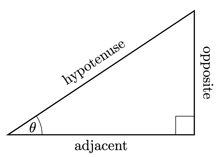
Definition 1. Consider the following right-angled triangle with acute angle $\theta \in (0, \pi/2)$ . Here and subsequently, we adopt the radian notation for angles that stipulates $2\pi = 360^{\circ}$ .

We abbreviate the words opposite, adjacent, and hypotenuse. We define the sine, cosine, and tangent of $\theta$ as follows:

$\begin{aligned} \sin(\theta) := \frac{\text{opp}}{\text{hyp}}, \quad \cos(\theta) := \frac{\text{adj}}{\text{hyp}}, \quad \tan(\theta) := \frac{\text{opp}}{\text{adj}}. \end{aligned}$

Example 1. By considering the $1$ – $\sqrt{3}$ – $2$ and $1$ – $1$ – $\sqrt 2$ right triangles, we have the following trigonometric ratios for special angles:

$\begin{aligned}\theta = \pi/6:&\quad \sin(\pi/6) = \frac{1}2,\quad \cos(\pi/6) = \frac {\sqrt{3}}2,\quad \tan(\pi/6) = \frac 1{\sqrt 3}. \\ \theta = \pi/4:&\quad \sin(\pi/4) = \frac 1{\sqrt 2},\quad \cos(\pi/4) = \frac 1{\sqrt 2} ,\quad \tan(\pi/4) = 1. \\ \theta = \pi/3:&\quad \sin(\pi/3) = \frac {\sqrt 3}2,\quad \cos(\pi/3) = \frac 12,\quad \tan(\pi/3) = \sqrt 3.\end{aligned}$

The case $\theta = \pi/4$ will play a crucial role for us later. Denote $\sin^2(\theta) := (\sin(\theta))^2$ for brevity. We will not care too much about the tangent function, since it is connected to sine and cosine in the following way:

Theorem 1. Let $\theta \in (0, \pi/2)$ . Then

$\displaystyle \sin^2(\theta) + \cos^2(\theta) = 1,\quad \tan(\theta) = \frac{\sin(\theta)}{\cos(\theta)},\quad \cos(\theta) = \sin(\pi/2 - \theta).$

Proof. For the first identity, use Pythagoras’ theorem to obtain

$\displaystyle \sin^2(\theta) + \cos^2(\theta) = \frac{\text{opp}^2}{\text{hyp}^2} + \frac{\text{adj}^2}{\text{hyp}^2} = \frac{\text{opp}^2 + \text{adj}^2}{\text{hyp}^2} = \frac{\text{hyp}^2}{\text{hyp}^2} = 1.$

For the second identity, we observe that

$\displaystyle \frac{\sin(\theta)}{\cos(\theta)} = \frac{\text{hyp} \cdot \sin(\theta)}{\text{hyp} \cdot \cos(\theta)} = \frac{\text{opp}}{\text{adj}} = \tan(\theta).$

For the last identity, since the complementary angle is $\pi/2-\theta$ ,

$\displaystyle \sin(\pi/2 - \theta) = \frac{\text{adj}}{\text{hyp}} = \cos(\theta).$

Strictly speaking, the cosine function is effectively a mutation of the sine function, and so we could technically do all of trigonometry in terms of sine. However, cosine does have its uses and will play a crucial role in our discussions moving forward.

There are many trigonometric identities built off the first two identities, and we will leave them as exercises in algebraic manipulation. For a serious study of trigonometry, we have to ask the all-important question: what is $\sin(\theta)$ if $\theta$ is not acute? In particular, what is a sensible definition for $\sin(\pi/2)$ ? The answer to the latter question turns out to answer the former question.

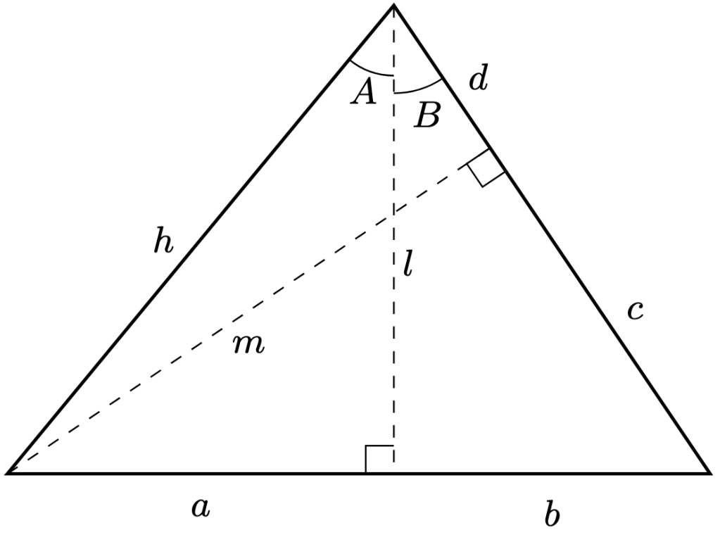
Theorem 2. Let $A,B$ be acute angles. If $A + B$ is acute, then

$\begin{aligned} \sin(A+B) &= \sin(A) \cos(B) + \cos(A) \sin(B), \\ \cos(A + B) &= \cos(A) \cos(B) - \sin(A) \sin(B). \end{aligned}$

Proof. Consider the following diagram for the proof of both identities.

The first identity corresponds to finding an alternate expression for $\sin(A+B) = m/h$ , and the second identity corresponds to finding an alternate expression for $\cos(A+B) = d/h$ . The ratios of interest are

$\displaystyle \sin(A) = \frac ah,\quad \cos(A) = \frac lh,\quad \sin(B) = \frac b{c+d},\quad \cos(B) = \frac l{c+d}.$

By considering the area of the whole triangle using the bases $(a+b)$ and $(c+d)$ respectively,

$\frac 12 \cdot (c + d)\cdot m = \frac 12 \cdot a\cdot l + \frac 12 \cdot b\cdot l.$

Dividing by $\frac 12 (c+d)h$ on both sides,

$\displaystyle \frac mh = \frac ah \cdot \frac l{c+d} + \frac lh \cdot \frac b{c+d}.$

By basic trigonometric ratios,

$\sin(A+B) = \sin(A) \cos(B) + \cos(A) \sin(B).$

For the second identity, by the Pythagorean theorem,

$(a+b)^2 - c^2 = m^2 = h^2 - d^2.$

By algebruh,

$c^2 = ((c+d) - d)^2 = (c+d)^2 - 2(c+d)d + d^2.$

Therefore,

$(a^2 + 2ab + b^2) - (c+d)^2 + 2(c+d)d - d^2 = h^2 - d^2.$

Simplifying the equation,

$2(c+d)d = (h^2 - a^2) + ((c+d)^2 - b^2) - 2ab.$

By Pythagoras’ theorem, $h^2 - a^2 = (c+d)^2 - b^2 = l^2$ , so that

$2(c+d)d =2l^2 - 2ab.$

Dividing by $2(c+d)h$ on both sides,

$\displaystyle \frac dh = \frac{l}{h} \cdot \frac{l}{c+d} - \frac{a}{h} \cdot \frac{b}{c+d}.$

By basic trigonometric ratios,

$\cos(A+B) = \cos(A) \cos(B) - \sin(A) \sin(B).$

Corollary 1. Let $\theta$ be acute. If $2\theta$ is acute, then

$\begin{aligned} \sin(2\theta) = 2\sin(\theta) \cos(\theta), \quad \cos(2\theta) = \cos^2(\theta) - \sin^2(\theta). \end{aligned}$

Proof. Set $A = B = \theta$ in Theorem 2.

The key insight is the following: as long as the right-hand side is well-defined, so is the left-hand side. This is our strategy to define $\sin$ and $\cos$ on all of $\mathbb R$ . Let’s systematise our plan.

Definition 1. For any subset $I \subseteq \mathbb R$ , let $\phi(I)$ be the proposition that for any $A, B \in I$ , $\sin(A+B)$ and $\cos(A + B)$ are well-defined, and

$\begin{aligned} \sin(A+B) &= \sin(A) \cos(B) + \cos(A) \sin(B), \\ \cos(A + B) &= \cos(A) \cos(B) - \sin(A) \sin(B). \end{aligned}$

Write $\phi(I)$ to abbreviate the proposition “ $\phi(I)$ is true”. Our overarching goal is to provide sensible definitions for $\sin$ and $\cos$ such that $\phi(\mathbb R)$ . By Theorem 1, we have established $\phi((0, \pi/8])$ and Corollary 1 will help us “double” our results to achieve the massive sub-goal of $\phi(\mathbb R^+)$ .

Theorem 3. For any $a > 0$ , suppose $\sin$ and $\cos$ are well-defined on $(0, 2a]$ . For any $\theta \in (0, 4a]$ , denote $\theta_2 := \theta/2 \in (0, 2a]$ and define

$\sin(\theta) := 2 \sin(\theta_2) \cos(\theta_2),\quad \cos(\theta) := \cos^2(\theta_2) - \sin^2(\theta_2).$

If $\phi((0, a])$ , then $\phi((0, 2a])$ .

Proof. Fix $A,B \in (0, 2a]$ . Then $A+B \in (0, 4a]$ . Observe that

$(A+B)_2 = A_2 + B_2 \in (0, 2a],$

so that $A_2,B_2 \in (0, a]$ and

$\begin{aligned} \sin(A+B) &= 2 \sin(A_2 + B_2) \cos(A_2 + B_2).\end{aligned}$

Since $\phi((0, a])$ , expanding the right-hand side yields

$\begin{aligned}\sin(A_2 + B_2) &= \sin(A_2) \cos(B_2) + \cos(A_2) \sin(B_2), \\ \cos(A_2 + B_2) &= \cos(A_2) \cos(B_2) - \sin(A_2) \sin(B_2).\end{aligned}$

On the other hand,

$\begin{aligned} \sin(A)\cos(B) &= 2 \sin(A_2)\cos(A_2) (\cos^2(B_2) - \sin^2(B_2)), \\ \sin(B)\cos(A) &= 2 \sin(B_2)\cos(B_2) (\cos^2(A_2) - \sin^2(A_2)). \end{aligned}$

With careful algebraic expansion, we will obtain

$\sin(A + B) = \sin(A)\cos(B) + \cos(A) \sin(B).$

Similarly, we will obtain

$\cos(A + B) = \cos(A) \cos(B) - \sin(A) \sin(B).$

Corollary 2. $\phi(\mathbb R^+)$ . In particular, we have the following special angles:

$\begin{aligned} \theta = \pi/2:&\quad \sin(\pi/2) = 1,\quad \cos(\pi/2) = 0 \\ \theta = \pi:&\quad \sin(\pi) = 0,\quad \cos(\pi) = -1. \\ \theta = 2\pi:&\quad \sin(2\pi) = 0,\quad \cos(2\pi) = 1.\end{aligned}$

Proof. Fix $A,B \in \mathbb R^+$ . Then there exists $N \in \mathbb N$ such that $A+B \in (0, 2^N \cdot \pi/8]$ . Using induction, we can prove that $\phi((0, 2^N \cdot \pi/8])$ . Therefore, $\sin, \cos$ are well-defined on $\mathbb R^+$ and the identities

$\begin{aligned} \sin(A+B) &= \sin(A) \cos(B) + \cos(A) \sin(B), \\ \cos(A + B) &= \cos(A) \cos(B) - \sin(A) \sin(B), \end{aligned}$

hold for any $A, B \in \mathbb R^+$ . Hence, $\phi(\mathbb R^+)$ , as required.

Corollary 3. For any $\theta > 0$ ,

$\sin(\theta + 2\pi) = \sin(\theta),\quad \cos(\theta + 2\pi) = \cos(\theta).$

Furthermore, for any positive integer $n$ ,

$\sin(\theta + n \cdot 2\pi) = \sin(\theta),\quad \cos(\theta + n \cdot 2\pi) = \cos(\theta).$

We have done a remarkable task: defining $\sin, \cos$ on $\mathbb R^+$ and proving that they satisfy the desired addition formulae. But we haven’t proven this case for all of $\mathbb R$ , since $\mathbb R = \mathbb R^- \sqcup \{0\} \sqcup \mathbb R^+$ . Surprisingly, though, Corollary 3 gives us a unique insight. Observe that for $\theta \in (-2\pi, 0]$ , $\sin(\theta +2\pi)$ and $\cos(\theta + 2\pi)$ are well-defined expressions. This means we can do a “reverse” definition for non-positive $\theta$ .

Theorem 4. For any $\theta \leq 0$ , let $n_\theta$ denote any integer such that $\theta + n_\theta \cdot 2\pi > 0$ . The notions

$\sin(\theta) := \sin(\theta + n_\theta \cdot 2\pi),\quad \cos(\theta) := \cos(\theta + n_\theta \cdot 2\pi)$

are well-defined by Corollary 3. Then $\phi(\mathbb R)$ . In particular,

$\sin(0) = \sin(2\pi) = 0,\quad \cos(0) = \cos(2\pi) = 1.$

Proof. Fix $A, B \in \mathbb R$ . Find $n_A, n_B \in \mathbb N$ such that $A +n_A \cdot 2\pi > 0$ and $B+n_B \cdot 2\pi > 0$ . Then $(A+B) + (n_A + n_B) \cdot 2\pi > 0$ so that $\phi(\mathbb R^+)$ allows

$\begin{aligned} \sin(A+B) &= \sin((A+B) + (n_A + n_B) \cdot 2\pi) \\ &= \sin((A + n_A \cdot 2\pi) + (B + n_B \cdot 2\pi)) \\ &= \sin(A + n_A \cdot 2\pi) \cos(B + n_B \cdot 2\pi) \\ &\phantom{==} + \cos(A + n_A \cdot 2\pi) \sin(B + n_B \cdot 2\pi) \\ &= \sin(A) \cos(B) + \cos(A) \sin(B). \end{aligned}$

A similar calculation yields

$\cos(A + B) = \cos(A) \cos(B) - \sin(A) \sin(B).$

Thus, we have properly defined $\sin$ and $\cos$ on all of $\mathbb R$ , and even proved that the identities

$\begin{aligned} \sin(A+B) &= \sin(A) \cos(B) + \cos(A) \sin(B), \\ \cos(A + B) &= \cos(A) \cos(B) - \sin(A) \sin(B), \end{aligned}$

are well-defined and hold for any $A, B \in \mathbb R$ . From these two key identities, we obtain all other trigonometric identities commonly obtained in tables of mathematical formulas.

—Joel Kindiak, 4 Jun 25, 1758H

August 31, 2025
An Inequality Puzzle

Problem 1. Suppose $f : \mathbb R \to \mathbb R$ satisfies the inequality

$\displaystyle |f(x) - f(y)| \leq (x-y)^2, \quad x ,y \in \mathbb R,$

and $f(0) = 1$ . Given $x \in \mathbb R$ , evaluate $f(x)$ .

(Click for Solution)

Solution. Fix $c \in \mathbb R$ . For any $h \in \mathbb R$ ,

$\displaystyle |f(c+h) - f(c)| \leq ((c+h)-c)^2 = h^2.$

Dividing by $|h|$ on both sides,

$\displaystyle \left| \frac{f(c+h) - f(c)}{h} \right| \leq |h|.$

Taking $h \to 0$ , by the squeeze theorem,

$\displaystyle f'(c) = \lim_{h \to 0} \frac{f(c+h) - f(c)}{h} = 0.$

Since $c \in \mathbb R$ is arbitrary, $f' = 0$ . Thus, $f$ is differentiable on $\mathbb R$ with derivative $f' = 0$ . Fix $x \in \mathbb R$ . By the mean value theorem, there exists $\xi$ between $0$ and $x$ such that

$f(x) = f(0) + f'(\xi) \cdot (x-0) = 1 + 0 \cdot x = 1.$

—Joel Kindiak, 23 Aug 25, 2237H

August 23, 2025
Classical Optimisation
Problem 1. Let $f$ be a non-negative function satisfying the following conditions:
- $f$ is continuous on $\mathbb R$ ,
- $f$ is differentiable on $\mathbb R \backslash \{0\}$ ,
- $f$ is strictly increasing on $(-\infty, 0)$ ,
- $f$ is strictly decreasing on $(0, \infty)$ , and
- $f(|x|) \to 0$ as $x \to \infty$ .
Let $A(x)$ denote the rectangle under the curve $y=f(x)$ whose base that intersects the positive $x$ -axis has length $x$ . If $A$ has a minimum prove that $A$ is minimised when

$\begin{aligned} \left( 1 - \frac { f'(x) }{(g' \circ g^{-1} \circ f)(x)} \right) \cdot f(x) + (x - (g^{-1} \circ f)(x)) \cdot f'(x) &= 0, \end{aligned}$

where $g = f|_{(-\infty, 0)}$ .

(Click for Solution)

Solution. Fix $c > 0$ . If $f(c) = 0$ , then $f$ being strictly decreasing implies $f(c+1) < 0$ , a contradiction. Therefore, $f(0) > f(c) > 0$ . Since $f(-x) \to 0$ as $x \to \infty$ , there exists $b \in (-\infty, 0)$ such that $f(b) < f(c) < f(0)$ . Use the intermediate value theorem to obtain $a \in (b, 0)$ such that $f(a) = f(c)$ . It is not hard to verify that $f(x) > f(c)$ for $x \in [a, c]$ . Therefore, the rectangle has an area $A(c)$ of $A(c) = (c - a) \cdot f(c)$ .

In fact, more is true. Since $g := f|_{(-\infty, 0)}$ is differentiable and strictly decreasing,

$g(a) = f(a) = f(c)\quad \Rightarrow \quad a = g^{-1}(f(c)).$

Hence, $A(x) = (x - (g^{-1} \circ f)(x) ) \cdot f(x)$ . Differentiating,

$\begin{aligned} A'(x) &= (1 - (g^{-1})'(f(x)) \cdot f'(x)) \cdot f(x) + (x - (g^{-1} \circ f)(x) ) \cdot f'(x) \\ &= \left( 1 - \frac { f'(x) }{g'((g^{-1} \circ f)(x))} \right) \cdot f(x) + (x - (g^{-1} \circ f)(x)) \cdot f'(x).\end{aligned}$

Setting $A' = 0$ yields the desired result.

Problem 2. Suppose further in Problem 1 that $f$ is even. Prove that the $x$ -value $x_0$ that maximises $A$ satisfies the equation

$f(x_0) + x_0 \cdot f'(x_0) = 0$

and the inequality

$2f'(x_0) + x_0 \cdot f''(x_0) < 0.$

Furthermore, the maximum area is given by $A(x_0) = 2x_0 \cdot f(x_0)$ .

(Click for Solution)

Solution. If $f$ is even, then for any $x > 0$ ,

$\displaystyle (g^{-1} \circ f)(x) = g^{-1}(f(x)) = f^{-1}(f(-x)) = -x,$

Furthermore, $f'$ is odd:

$\displaystyle f'(-x)\cdot(-1) = \frac{\mathrm d}{\mathrm dx} (f(-x)) = \frac{\mathrm d}{\mathrm dx}(f(x)) = f'(x),$

so that $f'(-x) = -f'(x)$ . Therefore, for any $x < 0$ , $g(x) = f(x) = f(-x)$ and

$g'(x) = f'(-x) \cdot (-1) = f'(x).$

Hence, for any $x > 0$ ,

$\begin{aligned} (g' \circ g^{-1} \circ f)(x) &= f' ((g^{-1} \circ f)(x)) \\ &= f'(-x) = -f'(x) \neq 0. \end{aligned}$

Substituting into the result in Problem 1,

$\begin{aligned} \left( 1 - \frac { f'(x) }{-f'(x)} \right) \cdot f(x) + (x - (-x)) \cdot f'(x) &= 0, \end{aligned}$

yielding $f(x) + x \cdot f'(x) = 0$ . For the inequality, apply the second derivative test.

Problem 3. Evaluate the maximum area of the rectangle defined in Problem 1 given that $f(x) = 1/( 1+x^2 )$ .

(Click for Solution)

Solution. For $x > 0$ , $f(x) = 1/( 1+x^2 )$ so that

$\displaystyle f'(x) = -\frac 1{( 1+x^2 )^2} \cdot 2x = -\frac{2x}{( 1+x^2 )^2}.$

Since $f$ is even, by Problem 2,

$\displaystyle \begin{aligned} \frac 1{1+x_0^2 } + x_0 \cdot \left( -\frac{2x_0}{ (1+x_0^2)^2 } \right) &= 0 \\ 1+x_0^2 + x_0 \cdot (-2x_0) &= 0\\ 1 - x_0^2 &= 0\\ x_0 &= 1, \end{aligned}$

since $x_0 = 1$ . To verify that this value gives the maximum, we evaluate the second derivative:

$\displaystyle f''(x) = 2 \cdot \frac{x^2 -1 }{(1+x^2)^4}\quad \Rightarrow \quad f''(x_0) = 0.$

Then $f'(x_0) = -1$ and $f''(x_0) = 0$ , so that

$2 \cdot f'(x_0) + f''(x_0) = -2 < 0,$

as required. Therefore, $f(x_0) =1/2$ and the maximum area is given by

$A(x_0) = 2 \cdot 1 \cdot f(1) = 1.$

—Joel Kindiak. 9 Aug 25, 1510H
August 9, 2025
Odd and Even Functions
Recall that $\sin(-x) = -\sin(x)$ and $\cos(-x) = \cos(x)$ for any $x \in \mathbb R$ .

Definition 1. For any function $f : \mathbb R \to \mathbb R$ , define $\tilde f : \mathbb R \to \mathbb R$ by $\tilde f(x) := f(-x)$ .

Problem 1. Given functions $f, g: \mathbb R \to \mathbb R$ , define $h_1 := f + g$ and $h_2 := f \cdot g$ . Prove that $\tilde h_1 = \tilde f + \tilde g$ and $\tilde h_2 = \tilde f \cdot \tilde g$ .

(Click for Solution)

Solution. By definition,

$\begin{aligned} \tilde h_1(x) = h_1(-x) &= (f+g)(-x) \\ &= f(-x) + g(-x) \\ &= \tilde f(x) + \tilde g(x) \\ &= (\tilde f + \tilde g)(x), \end{aligned}$

and

$\begin{aligned} \tilde h_2(x) = h_2(-x) &= (f \cdot g)(-x) \\ &= f(-x) \cdot g(-x) \\ &= \tilde f(x) \cdot \tilde g(x) \\ &= (\tilde f \cdot \tilde g)(x). \end{aligned}$

Definition 2. A function $f : \mathbb R \to \mathbb R$ is odd (resp. even) if there exists an odd (resp. even) integer $n$ such that $\tilde f = (-1)^n \cdot f$ .

Example 1. For any integer $n$ , the function $f_n$ defined by $f_n(x) = x^n$ is an odd (resp. even) function if and only if $n$ is an odd (resp. even) number. Furthermore, $\sin$ is an odd function while $\cos$ is an even function.

Problem 2. For any function $f: \mathbb R \to \mathbb R$ and real number $\alpha \in \mathbb R$ , define the function $f_\alpha$ by $f_\alpha(x) := f(\alpha x)$ . In particular, $f_{-1} = \tilde f$ . Prove that $f_\alpha$ is odd (resp. even) if $f$ is odd (resp. even).

(Click for Solution)

Solution. We observe that if $f$ is odd or even, then $\tilde f = (-1)^n f$ , so that

$\begin{aligned} \tilde f_\alpha(x) &= f_\alpha(-x) = f(\alpha(-x))= f(-(\alpha x)) \\ &= \tilde f(\alpha x) = (-1)^n \cdot f(\alpha x) = (-1)^n \cdot f_\alpha(x), \end{aligned}$

hence $\tilde f_\alpha= (-1)^n \cdot f_\alpha$ .

Problem 3. Prove the following properties:
- if $f, g$ are odd, then $f + g$ is odd and $f \cdot g$ is even,
- if $f, g$ are even, then $f + g$ is even and $f \cdot g$ is even,
- if $f$ is odd and $g$ is odd (resp. even), then $g \circ f$ is odd (resp. even) whenever it exists.
- if $f$ is even, then $g \circ f$ is even.
(Click for Solution)

Solution. Suppose $\tilde f = (-1)^m \cdot f$ and $\tilde g = (-1)^n \cdot g$ , and assume $m \leq n$ for simplicity. Denote $h_1 = f+g$ and $h_2 = f \cdot g$ as per Problem 1. Then

$\tilde h_1 = \tilde f + \tilde g = (-1)^m \cdot f + (-1)^n \cdot g = (-1)^m \cdot (f + (-1)^{n-m} \cdot g).$

If $m$ and $n$ are both odd or both even, then $n-m$ is even, so that

$\tilde h_1 = (-1)^m \cdot (f + g) = (-1)^m \cdot h_1.$

Hence, $h_1$ is odd (resp. even) if and only if $f$ is odd (resp. even). Similarly,

$\tilde h_2 = \tilde f \cdot \tilde g = (-1)^m \cdot f \cdot (-1)^n \cdot g = (-1)^{m+n} \cdot h_2.$

If $m$ and $n$ are both odd or both even, then $m+n$ is always even, so that $\tilde h_2 = h_2$ unconditionally, i.e. $h_2 = f \cdot g$ is even. For the composite function, define $h_3 := g \circ f$ . Then

$\tilde h_3(x) = h_3(-x) = (g \circ f)(-x) = g(f(-x)) = g(\tilde f(x)) = (g \circ \tilde f)(x).$

Applying the odd or even condition on $f$ ,

$\begin{aligned} g \circ \tilde f &= g \circ (-(-1)^{m+1} \cdot f) \\ &= \tilde g \circ ((-1)^{m+1} \cdot f) \\ &= (-1)^n \cdot g \circ ((-1)^{m+1} \cdot f). \end{aligned}$

If $f$ is odd, then $m + 1$ is even, so that

$\tilde h_3 = g \circ \tilde f = (-1)^n \cdot (g \circ f) = (-1)^n \cdot h_3.$

Thus, $h_3$ is odd (resp. even) if and only if $g$ is odd (resp. even). If $f$ is even, then

$\tilde h_3 = g \circ \tilde f = g \circ f = h_3,$

so that $h_3$ is even.

Problem 4. For any function $f: \mathbb R \to \mathbb R$ , prove that there exist a unique odd function $f_1$ and a unique even function $f_2$ such that $f = f_1 + f_2$ .

(Click for Solution)

Solution. For existence, define the functions $f_1, f_2$ by

$f_1 := \frac 12 \cdot (f - \tilde f),\quad f_2 := \frac 12 \cdot (f + \tilde f).$

It is obvious that $f = f_1 + f_2$ . Since $\tilde{ \tilde f } = f$ ,

$\begin{aligned} \tilde f_1 &= \textstyle \frac 12 \cdot (\tilde f - \tilde{ \tilde f }) = \frac 12 \cdot (\tilde f - f) = -f_1, \\ \tilde f_2 &= \textstyle \frac 12 \cdot (\tilde f + \tilde{ \tilde f }) = \frac 12 \cdot (\tilde f + f) = f_2, \end{aligned}$

so that $f_1$ is odd and $f_2$ is even. For uniqueness, suppose $f = f_1 + f_2 = \hat f_1 + \hat f_2$ , where $\hat f_1$ is odd and $\hat f_2$ is even. Then $g := f_1 - \hat f_1 = \hat f_2 - f_2$ , so that $g$ is both odd and even. Hence,

$g = \tilde g = -g \quad \Rightarrow \quad g = 0\quad \Rightarrow \quad \hat f_1 = f_1\quad \Rightarrow \quad \hat f_2 = f_2.$

Problem 5. Fix $a > 0$ , any odd continuous function $f_1$ , and any even continuous function $f_2$ . Prove that

$\displaystyle \int_{-a}^a f_1 (x)\,\mathrm dx = 0, \quad \int_{-a}^a f_2 (x)\,\mathrm dx = 2 \cdot \int_0^a f_2 (x)\,\mathrm dx.$

In particular, for any continuous function $f : \mathbb R \to \mathbb R$ ,

$\displaystyle \int_{-a}^a f (x)\,\mathrm dx = 2 \cdot \int_0^a f_2 (x)\,\mathrm dx.$

(Click for Solution)

Solution. Using a substitution,

$\displaystyle \int_{-a}^0 f_1(x)\, \mathrm dx = \int_{a}^0 f_1(-t)\cdot (-1)\, \mathrm dt = \int_0^a -f_1(t)\, \mathrm dt = - \int_0^a f_1(t)\, \mathrm dt.$

Therefore,

$\displaystyle \begin{aligned} \int_{-a}^a f_1 (x)\,\mathrm dx &= \int_{-a}^0 f_1(x)\, \mathrm dx + \int_0^a f_1(x)\, \mathrm dx = 0.\end{aligned}$

Similarly, we can prove that

$\displaystyle \int_{-a}^0 f_2(x)\, \mathrm dx = \int_0^a f_2(t)\, \mathrm dt$

so that

$\displaystyle \begin{aligned} \int_{-a}^a f (x)\,\mathrm dx &= \int_{-a}^0 f_2(x)\, \mathrm dx + \int_0^a f_2(x)\, \mathrm dx = 2 \cdot \int_0^a f_2(x)\, \mathrm dx.\end{aligned}$

Problem 6. For any continuous function $f : \mathbb R \to \mathbb R$ and $T > 0$ , define

$\displaystyle a_n := \frac 2T \int_{-T/2}^{T/2} f(t)\, \mathrm \cos \left( \frac{2n \pi t}{T} \right)\, \mathrm dt,\quad b_n := \frac 2T \int_{-T/2}^{T/2} f(x)\, \mathrm \sin \left( \frac{2n \pi t}{T} \right)\, \mathrm dt.$

Prove that $a_n = 0$ (resp. $b_n = 0$ ) if $f$ is odd (resp. even).

(Click for Solution)

Solution. By Example 1 and Problem 2, $\cos_{2n\pi/T}$ is even and $\sin_{2n\pi/T}$ is odd.

Thus, if $f$ is odd, then $f \cdot \cos_{2n\pi/T}$ is odd by Problem 3, so that $a_n = 0$ by Problem 5.

Similarly, if $f$ is even, then $f \cdot \sin_{2n\pi/T}$ is odd by Problem 3, so that $b_n = 0$ by Problem 5.

—Joel Kindiak, 5 Aug 25, 2044H
August 5, 2025
Some Calculus of Variations

Problem 1. Let $f : (a, b) \to \mathbb R$ be continuous. Prove that if $f \neq 0$ , then there exists $c, d \in (a, b)$ such that $\pm f(x) > 0$ whenever $x \in (c, d)$ .

(Click for Solution)

Solution. Suppose $f(x_0) \neq 0$ for some $x_0 \in (a, b)$ . Then $f(x_0) > 0$ or $f(x_0) < 0$ . In the case $f(x_0) > 0$ , use the continuity of $f$ to find $\delta \in (0, \min\{x_0-a, b-x_0\})$ such that

$\displaystyle |x - x_0| < \delta \quad \Rightarrow \quad |f(x) - f(x_0)| < \frac{f(x_0)}{2}.$

By expanding the inequality,

$\displaystyle f(x) - f(x_0) > -\frac{f(x_0)}{2} \quad \Rightarrow \quad f(x) > \frac{f(x_0)}{2} > 0.$

Defining $c := x_0 - \delta$ and $d:= x_0 + \delta$ ,

$x \in (c, d) \quad \Rightarrow \quad |x - x_0| < \delta \quad \Rightarrow \quad f(x) > 0.$

In the case $f(x_0) < 0$ , we have $(-f)(x_0) > 0$ . Applying the first case, there exists $c, d \in (a, b)$ such that

$x \in (c, d) \quad \Rightarrow \quad -f(x) = (-f)(x) > 0.$

Problem 2. Let $f : (a, b) \to \mathbb R$ be continuous and suppose $f(x) \geq 0$ for any $(a, b)$ . Prove that

$\displaystyle \int_a^b f(x)\, \mathrm dx = 0 \quad \Rightarrow \quad f = 0.$

(Click for Solution)

Solution. Suppose instead that $f \neq 0$ . Then there exists $(c, d) \subseteq (a, b)$ such that for any $x \in (c, d)$ , $f(x) > 0$ . Hence,

$\begin{aligned} \int_a^b f(x)\, \mathrm dx &= \int_a^c f(x)\, \mathrm dx + \int_c^d f(x)\, \mathrm dx + \int_d^b f(x)\, \mathrm dx \\ &\geq 0 + \int_c^d f(x)\, \mathrm dx + 0\\ &= \int_c^d f(x)\, \mathrm dx > 0 . \end{aligned}$

Definition 1. Call a function $h \in C^\infty$ compactly supported if there exists real numbers $c < d$ such that $h(x) = 0$ for $x \leq c$ and $x \geq d$ .

Problem 3. Let $f : (a, b) \to \mathbb R$ be continuous. Suppose that for any compactly supported $h$ ,

$\displaystyle \int_a^b f(x)h(x)\, \mathrm dx = 0.$

Then $f = 0$ .

(Click for Solution)

Solution. By way of contradiction, suppose $f \neq 0$ . By Problem 1, there exists $(c, d) \subseteq (a, b)$ such that without loss of generality, $f(x) > 0$ whenever $x \in (c, d)$ . Define $h \in C^\infty$ by

$h(x) = \begin{cases} e^{ -\frac{1}{ (x-c)(d-x) } }, & x \in (c, d), \\ 0, & \text{otherwise}.\end{cases}$

Then it is clear that $h$ is compactly supported, and that for any $x \in (a, b)$ , $f(x)h(x) \geq 0$ . By Problem 2, $f \cdot h = 0$ . However for $m := (c+d)/2$ ,

$0 = (f \cdot h)(m) = f(m) \cdot h(m) > 0 \cdot 0 = 0,$

a contradiction.

—Joel Kindiak, 25 Jun 25, 1420H

June 25, 2025
Curious Continuity

Problem 1. Define the function $f : [-1, 1] \to \mathbb R$ by

$f(x) = \begin{cases} x^2, & x \in [-1,1] \cap \mathbb Q, \\ -x^2, & x \in [-1,1] \backslash \mathbb Q. \end{cases}$

Prove that $f$ is continuous at $0$ .

(Click for Solution)

Solution. We observe that $-x^2 \leq f(x) \leq x^2$ . Since $\pm x^2 \to 0$ as $x \to 0$ , by the squeeze theorem, $f(x) \to 0 = 0^2 = f(0)$ as $x \to 0$ , as required.

Problem 2. For any function $f$ that is continuous at $c$ , prove that if $f(c) > 0$ , then there exists $\delta > 0$ such that for $x \in (c - \delta, c + \delta)$ , $f(x) > 0$ .

(Click for Solution)

Solution. Suppose $f(c) > 0$ . Fix $\epsilon > 0$ that will be chosen later. Since $f$ is continuous at $c$ , for any $k > 0$ , there exists $\delta > 0$ such that

$|x-c| < \delta \quad \Rightarrow \quad |f(x) - f(c)| < k \cdot \epsilon.$

Expanding the right-hand side, $f(x) > f(c) - k \cdot \epsilon$ . Setting $\epsilon = f(c) > 0$ and $k = 1/2$ ,

$\displaystyle f(x) > f(c) - \frac{1}{2} \cdot f(c) = \frac{f(c)}{2} > 0.$

Problem 3. Let $f : [a, b] \to \mathbb R$ be continuous. Suppose that for any $x \in [a, b]$ , $f(x) \neq 0$ . Prove that there exists $C > 0$ such that either $f < -C$ or $f > C$ . In particular, $|f| > C$ .

(Click for Solution)

Solution. The function $g := | \cdot | \circ f : [a, b] \to \mathbb R$ is a composition of continuous functions and thus continuous. By the extreme value theorem, there exists $c \in [a, b]$ such that for any $x \in [a, b]$ ,

$|f(x)| = g(x) \geq g(c) = |f(c)|.$

Since $f(c) \neq 0$ , $|f(c)| > 0$ , so that defining $C := |f(c)| / 2 > 0$ yields

$|f(x)| \geq |f(c)| > C.$

Now suppose $f(c_0) > 0$ without loss of generality. In the case $f(c_0) < 0$ , apply the first case to the continuous map $-f$ . We claim that $f > 0$ .

Suppose, for a contradiction, there exists $c_1 \in (a, b)$ such that $f(c_1) < 0$ . Assume $c_1 \in (c_0, b)$ without loss of generality. By the intermediate value theorem, there exists $c_2 \in (c_0, c_1)$ such that $f(c_2) = 0$ , a contradiction. Therefore, $f > 0$ . For any $x \in [a, b]$ , $f(x) = |f(x)| > C$ , yielding $f > C$ , as required.

Problem 4. Let $f : \mathbb R \to \mathbb R$ and suppose that for any $x, y \in \mathbb R$ ,

$f(x + y) = f(x) + f(y).$

Prove that if $f$ is continuous at some $c \in \mathbb R$ , then $f$ is continuous on $\mathbb R$ .

(Click for Solution)

Fix $x \in \mathbb R$ . Since $f$ is continuous at $c$ ,

$\begin{aligned} f(c) &= \lim_{t \to 0} f(c+t) \\ &= \lim_{t \to 0} (f(c)+f(t)) \\ &= \lim_{t \to 0} f(c)+\lim_{t \to 0} f(t) \\ &= f(c) \cdot 1 + \lim_{t \to 0} f(t), \end{aligned}$

so that $\displaystyle \lim_{t \to 0}f(t) = 0$ . Therefore,

$\begin{aligned} \lim_{t \to 0} f(x+t) &= \lim_{t \to 0} (f(x)+f(t)) \\ &= \lim_{t \to 0} f(x) + \lim_{t \to 0} f(t) \\ &= f(x) \cdot 1 + 0 = f(x). \end{aligned}$

Problem 5. Let $f : [0, 1] \to \mathbb R$ be continuous and $f(0) = f(1)$ . Prove that for any $n \in \mathbb N^+$ , there exists $\xi \in [0,1]$ such that $f(\xi+1/n) = f(\xi)$ .

(Click for Solution)

Solution. For each $n$ , define the function $g := f(\cdot + 1/n) - f$ . We aim to show that $g$ has at least one root. We claim that there exists $x_0 \in [0,1]$ such that $g(x_0) \geq 0$ . Otherwise, $f < f(\cdot + 1/n)$ . In particular,

$\displaystyle f(0) < f(1/n) < f(2/n) < \cdots < f(1) = f(0),$

a contradiction. Therefore, there exists $x_0 \in [0,1]$ such that $g(x_0) \geq 0$ . A similar argument shows that there exists $x_1 \in [0,1]$ such that $g(x_1) \leq 0$ .

If at least one equality holds, then set $\xi = x_0$ or $\xi = x_1$ . Otherwise, $g(x_0) > 0$ and $g(x_1) < 0$ . Use the intermediate value theorem to find $c$ between $x_0$ and $x_1$ such that $g(c) = 0$ , as required.

—Joel Kindiak, 16 Aug 25, 2039H

June 18, 2025
Exponential Fourier Series

The function $f$ is defined by $f(t) = e^t$ for $-1 < t \leq 1$ and extended periodically by $f(t) = f(t+2)$ .

Problem 1. For any nonnegative integer $n$ , evaluate the integrals

$\displaystyle \int f(t) \cos (n \pi t)\, \mathrm dt,\quad \int f(t) \sin(n \pi t)\, \mathrm dt.$

(Click for Solution)

Solution. Integrating by parts twice,

$\begin{aligned} \int e^{t} \cos (n \pi t)\, \mathrm dt &= \underbrace{e^t}_{\mathrm I} \cdot \underbrace{\cos (n \pi t)}_{\mathrm S} - \int \underbrace{e^t}_{\mathrm I} \cdot \underbrace{(-n\pi \cdot \sin(n \pi t))}_{\mathrm D}\, \mathrm dt \\ &= e^t \cos(n\pi t) + n \pi \int e^t \sin(n \pi t)\, \mathrm dt \\ &= e^t \cos(n \pi t) + n\pi \left( \underbrace{e^t}_{\mathrm I} \cdot \underbrace{\sin (n \pi t)}_{\mathrm S} - \int \underbrace{e^t}_{\mathrm I} \cdot \underbrace{(n\pi \cdot \cos(n \pi t))}_{\mathrm D}\, \mathrm dt \right) \\ &= e^t ( \cos(n \pi t) + n\pi \sin(n \pi t)) - n^2 \pi^2 \int e^t \cos(n\pi t)\, \mathrm dt. \end{aligned}$

By careful algebruh,

$\displaystyle \int e^{t} \cos (n \pi t)\, \mathrm dt = \frac{e^t ( \cos(n \pi t) + n\pi \sin(n \pi t))}{1 + n^2 \pi^2} + C_1.$

In a similar though tedious manner,

$\displaystyle \int e^{t} \sin (n \pi t)\, \mathrm dt = \frac{e^t ( \sin(n \pi t) - n\pi \cos(n \pi t))}{1 + n^2 \pi^2} + C_2.$

Remark 1. For an alternate solution, recall Euler’s formula which states that

$e^{i n \pi t} = \cos(n \pi t) + i \sin(n \pi t).$

Multiplying by $f(t)$ then integrating on the left-hand side yields

$\begin{aligned} \int f(t) e^{i n \pi t} \, \mathrm dt &= \int e^t \cdot e^{i n \pi t}\, \mathrm dt \\ &= \int e^{(1 + i n \pi )t}\, \mathrm dt \\ &= \frac {e^{(1 + i n \pi )t}}{1 + i n \pi} + C \\ &= e^t \cdot \frac{1 - i n \pi}{1 + n^2 \pi^2} (\cos (n \pi t) + i \sin(n \pi t)) + C \\ &= e^t \cdot \frac{(\cos (n \pi t) + n \pi \sin(n \pi t)) + i (\sin(n \pi t) - n \pi \cos(n \pi t))}{1 + n^2 \pi^2} + C \\ &= e^t \cdot \frac{\cos (n \pi t) + n \pi \sin(n \pi t)}{1 + n^2 \pi^2} + i \cdot e^t \cdot \frac{\sin(n \pi t) - n \pi \cos(n \pi t)}{1 + n^2 \pi^2} + C . \end{aligned}$

The real and imaginary parts then agree with our solutions in Problem 1.

Problem 2. Denoting $T = 2$ , the Fourier series of $f$ is defined by

$\displaystyle f(t) = \frac{a_0}{2} + \sum_{n=1}^\infty \left( a_n \cos\left( \frac{2n\pi t}{T} \right) + b_n \sin\left( \frac{2n\pi t}{T} \right) \right),$

where the Fourier coefficients $a_n, b_n$ are defined by

$\displaystyle a_n = \frac 2{T} \int_{-T/2}^{T/2} f(t) \cos\left( \frac{2n\pi t}{T} \right)\, \mathrm dt,\quad b_n = \frac 2{T} \int_{-T/2}^{T/2} f(t) \sin\left( \frac{2n\pi t}{T} \right)\, \mathrm dt.$

Use Problem 1 to evaluate the Fourier series of $f$ .

(Click for Solution)

Solution. By Problem 1,

$\begin{aligned} a_n &= \frac 2{2} \int_{-2/2}^{2/2} f(t) \cos \left( \frac{2n\pi t}{2} \right)\, \mathrm dt \\ &= \int_{-1}^1 e^t \cos (n \pi t)\, \mathrm dt \\ &= \left[ \frac{e^t ( \cos(n \pi t) + n\pi \sin(n \pi t))}{1 + n^2 \pi^2} \right]_{-1}^1 \\ &= \frac{(-1)^n ( e - e^{-1} )}{1 + n^2 \pi^2} . \end{aligned}$

Similarly,

$\begin{aligned} b_n &= \frac 2{2} \int_{-2/2}^{2/2} f(t) \sin \left( \frac{2n\pi t}{2} \right)\, \mathrm dt \\ &= \int_{-1}^1 e^t \sin (n \pi t)\, \mathrm dt \\ &= \left[ \frac{e^t ( \sin(n \pi t) - n\pi \cos(n \pi t))}{1 + n^2 \pi^2} \right]_{-1}^1 \\ &= -n \pi \cdot \frac {(-1)^n (e - e^{-1} )}{1 + n^2 \pi^2} = -n\pi a_n. \end{aligned}$

By the definition of the Fourier series,

$\displaystyle \begin{aligned} f(t) &= \frac{a_0}{2} + \sum_{n=1}^\infty \left( a_n \cos\left( \frac{2n\pi t}{T} \right) + b_n \sin\left( \frac{2n\pi t}{T} \right) \right) \\ &= \frac{a_0}{2} + \sum_{n=1}^\infty a_n (( \cos (n \pi t) - \pi n \sin (n \pi t) ) \\ &= \frac{e - e^{-1}}{2} + \sum_{n=1}^\infty \frac{(-1)^n ( e - e^{-1} )}{1 + n^2 \pi^2} (( \cos (n \pi t) - \pi n \sin (n \pi t) ). \end{aligned}$

Remark 2. If instead we used the complex-exponential form of the Fourier series

$\displaystyle f(t) = \sum_{n = -\infty}^\infty c_n e^{i \cdot 2\pi n t/T},\quad c_n := \frac 1{T} \int_{-T/2}^{T/2} f(t) \cdot e^{i \cdot 2\pi n t/T}\, \mathrm dt,$

then complex-valued integration yields

$\displaystyle c_n = \frac 12 \left[ \frac{e^{(1 + i \cdot \pi n) t}}{1 + i \cdot \pi n} \right]_{-1}^1 = \frac {(-1)^n (e - e^{-1})(1 - (\pi n) \cdot i)}{2(1 + n^2 \pi^2)},$

recovering the results in Problem 2 via the relationships

$a_n = c_n + \bar{c}_n,\quad b_n = -i \cdot (c_n - \bar{c}_n) =-n\pi a_n.$

—Joel Kindiak, 14 May 25, 1911H

May 14, 2025
Launching Calculus

A modern myth is that calculus began after an apple struck Sir Isaac Newton in the head. Whether this story is valid or not, one thing is certain—Newton’s curiosity into gravity and motion did in fact lead him to formulate what we now know as calculus.

Newton formulated three famous laws of motion, that applied to gravitational motion on earth. While exploring that area of study launches us into Newtonian mechanics, one thing we will mention is Newton’s insight into gravitational acceleration. At least on earth, and at least for sufficiently low heights, the gravitational acceleration $g \approx 9.81\ \text{m}/\text{s}$ is constant.

Let $a(t)$ denote the acceleration of an object in linear motion at time $t$ . Newton contemplated that the velocity $v(t)$ of the object can be obtained by summing up approximate accelerations in small units $\Delta t$ of time:

$\displaystyle v(t) \approx \sum a(t)\Delta t.$

Allowing the time intervals to approach $0$ , we obtain

$\displaystyle v(t) := v(0)+ \int_0^t a(u)\, \mathrm du.$

But velocity in turn can be conceptualised as small packets of changes in displacements (i.e. distances with direction), so that the displacement $s(t)$ can be defined by

$\displaystyle s(t) := s(0)+ \int_0^t v(u)\, \mathrm du.$

From these ideas we obtain the usual equivalent definitions of velocity and acceleration:

$\displaystyle \begin{aligned} v(t) &= s'(t) = \frac{\mathrm ds}{\mathrm dt}, \\ a(t) &= v'(t) = \frac{\mathrm d^2 s}{\mathrm dt^2}.\end{aligned}$

Theorem 1. Define $s,v$ as per the discussions above. Suppose $s(0) = s_0$ and $v(0) = v_0$ . Suppose $a(t) = a$ is constant. Then the following laws of kinematics hold:

$\begin{aligned}v(t) &= v_0 + at, \\ s(t) &= s_0 + v_0 t + \textstyle \frac 12 at^2 \\ v(t)^2 &= v_0^2 + 2a(s(t) - s_0). \end{aligned}$

Proof. By integration techniques,

$\begin{aligned} v(t) &= \int_0^t a(u)\, \mathrm du \\ &= \int_0^t a\, \mathrm du \\ &= v(0) + \left[au\right]_0^t \\ &= v_0 + at. \end{aligned}$

Integrating a second time,

$\begin{aligned} s(t) &= \int_0^t v(u)\, \mathrm du \\ &= \int_0^t (v_0 + au)\, \mathrm du \\ &= s(0) + \left[v_0 u + \textstyle \frac 12 au^2\right]_0^t \\ &= s_0 + v_0 t + \textstyle \frac 12 at^2. \end{aligned}$

Therefore,

$\begin{aligned}v(t)^2 &= (v_0 + at)^2 \\ &= v_0^2 + 2v_0 at + a^2 t^2 \\ &= \textstyle v_0^2 + 2a \left(v_0 t + \frac 12 a t^2 \right) \\ &= v_0^2 + 2a(s(t) - s_0).\end{aligned}$

It turns out that these laws of kinematics can be used to start wars, applied in the context of projectile motion. The question is simple: If we fired a cannonball with initial position $(0, y_0)$ , initial velocity $v_0$ , and initial angle $\theta$ to the horizontal ground, what will the cannon’s path look like?

Corollary 1. Assuming no air resistance, the horizontal displacement $x(t)$ and vertical displacement $y(t)$ are given by

$x(t) = v_0 \cos(\theta) t,\quad y(t) = y_0 + (v_0 \sin(\theta))t - \frac 12 gt^2,$

where $g \approx 9.81\ \text{m}/\text{s}^2$ denotes gravitational acceleration on earth. Furthermore, the path of the cannonball follows the shape of a parabola (i.e. the graph of a quadratic function).

Proof. The initial horizontal velocity is $v_0 \cos(\theta)$ and the horizontal acceleration is $0$ , so that by Theorem 1,

$x(t) = 0 + v_0 \cos(\theta) t + \frac 12 \cdot 0 \cdot t^2 = v_0 \cos(\theta) t.$

Similarly, the initial vertical velocity is $v_0 \sin(\theta)$ and the vertical acceleration is $-g$ , so that by Theorem 1,

$y(t) = y_0 + (v_0 \sin(\theta))t - \frac 12 gt^2.$

By algebraic manipulation,

$\displaystyle \begin{aligned} y &= y_0 + \frac{v_0 \sin(\theta)}{v_0 \cos(\theta)} x - \frac 12 g \left( \frac{x}{v_0 \cos(\theta)} \right)^2 \\ &= y_0 + \tan(\theta)x - \frac{g}{2 v_0^2 \cos^2(\theta)}x^2\end{aligned}$

is the graph of a quadratic equation.

Now, what about if air resistance is involved? Then we need to solve differential equations. Furthermore, since we need to account for both $x$ – and $y$ -directions, we’ll need a tinge of vector calculus to properly answer this question. However, for simplicity, let’s solve answer the question for vertical motion and assume $x(t) = 0$ .

Theorem 2. Let $v(t)$ denote the velocity of an object with mass $m$ dropped from rest after time $t$ (so that $v(0) = 0$ ). Let $k >0$ be a constant that quantifies the air resistance that opposes the object’s motion. Newton’s second law yields the equation

$\displaystyle m \frac{\mathrm dv}{\mathrm dt} = mg - kv.$

Then $v \to kg/m$ as $t \to \infty$ . This is known as the terminal velocity of the object.

Proof. Dividing by $m$ on both sides,

$\displaystyle \frac{\mathrm dv}{\mathrm dt} = g - \frac km v.$

Making the substitution $\displaystyle v = \frac mk u$ ,

$\displaystyle \frac mk \cdot \frac{\mathrm du}{\mathrm dt} = -(u-g).$

Dividing on both sides the integrating (this is known as the method of separable variables),

$\displaystyle \ln|u-g| = \int \frac 1{u-g}\, \mathrm du = \int -\frac km\, \mathrm dt = -\frac km t + C.$

Performing some algebra and denoting $A = \pm e^C$ ,

$u = g + Ae^{-\frac km t}.$

Therefore,

$\displaystyle v = \frac{k}{m} ( g + Ae^{-\frac km t} ).$

Since $v(0) = 0$ , we have $A = -g$ , so that

$\displaystyle v = \frac{kg}{m} (1- e^{-\frac km t}).$

Taking $t \to \infty$ yields $e^{-\frac km t} \to 0$ . Hence, $v \to kg/m$ , as required.

Kinematics therefore, in many ways, launched the study of calculus, pun intended.

—Joel Kindiak, 5 Mar 25, 1653H

April 22, 2025