Category: Differential Equations

Un-abusing the Product Rule

Problem 1. Given $f$ , solve the differential equation

$\displaystyle \frac{\mathrm d}{\mathrm dx}(y \cdot f(x)) = \frac{\mathrm dy}{\mathrm dx} \cdot f'(x).$

(Click for Solution)

Solution. Using the product rule correctly to expand the left-hand side,

$\displaystyle \frac{\mathrm d}{\mathrm dx}(y \cdot f(x)) = \frac{\mathrm dy}{\mathrm dx} \cdot f(x) + y \cdot f'(x).$

Therefore,

$\displaystyle \frac{\mathrm dy}{\mathrm dx} \cdot f(x) + y \cdot f'(x) = \frac{\mathrm dy}{\mathrm dx} \cdot f'(x).$

Making $\frac{\mathrm dy}{\mathrm dx}$ the subject,

$\begin{aligned} \frac 1y \cdot \frac{\mathrm dy}{\mathrm dx} = \frac{ f'(x) }{ f'(x) - f(x) }. \end{aligned}$

Therefore, integrating with respect to $x$ on both sides,

$\displaystyle \ln|y| = \int \frac{f'(x)}{f(x) - f'(x)}\, \mathrm dx.$

Problem 2. Deduce the solution to the differential equation

$\displaystyle \frac{\mathrm d}{\mathrm dx}((y^2+1) \cdot \sin(x)) = 2y \cdot \frac{\mathrm dy}{\mathrm dx} \cdot \cos(x).$

(Click for Solution)

Solution. Firstly, since $\frac{\mathrm d}{\mathrm dx}(y^2 + 1) = 2y \cdot \frac{\mathrm dy}{\mathrm dx}$ , setting $f(x) = \sin(x)$ in Problem 1 yields the solution

$\begin{aligned}\ln(y^2 + 1) &= \int \frac{\cos(x)}{ \cos(x) - \sin(x) }\, \mathrm dx. \end{aligned}$

Use trigonometric identities to simplify the integrand as follows:

$\begin{aligned} \frac{ \cos(x) }{ \cos(x) - \sin(x) } &= \frac{ \cos(x) }{ \cos(x) - \sin(x) } \cdot \frac{ \cos(x) + \sin(x) }{ \cos(x) + \sin(x) } \\ &= \frac{ \cos^2(x) + \sin(x) \cos(x) }{ \cos^2(x) - \sin^2(x) } \\ &= \frac{ \frac 12 (\cos(2x)+1) + \frac 12 \sin(2x) }{ \cos(2x) } \\ &= \frac 12 \cdot \left( 1 + 2\sec(2x) + \tan(2x) \right). \end{aligned}$

Therefore, integrating the right-hand side,

$\begin{aligned} \int \frac{ \cos(x) }{ \cos(x) - \sin(x) } \, \mathrm dx &= \frac 12 \cdot \int \left( 1 + 2\sec(2x) + \tan(2x) \right)\, \mathrm dx \\ &= \frac 12 \left( x + \ln|{\sec(2x) + \tan(2x)}| + \frac 12 \ln |{ \sec(2x) }| \right) + C \\ &= \frac 12 x + \frac 12 \ln|{\sec(2x) + \tan(2x)}| + \frac 14 \ln |{ \sec(2x) }| + C. \end{aligned}$

Therefore, the required solution is

$\displaystyle \ln(y^2 + 1) = \frac 12 x + \frac 12 \ln|{\sec(2x) + \tan(2x)}| + \frac 14 \ln |{ \sec(2x) }| + C.$

—Joel Kindiak, 1 Sept 2025, 1645H

February 6, 2026
Kindiak Gauntlet (Differential Equations)

Warning. All questions below are non-trivial.

Section A (48 marks)

Each question in this section is worth 8 marks.

Question 1. Solve the differential equation

$\displaystyle \frac{\mathrm dy}{\mathrm dx} = \frac{1 + 2y^2}{\sqrt{9 - 4x^2}}.$

(Click for Solution)

Solution. By the method of separable variables,

$\begin{aligned} \frac{1}{1 +2y^2} \cdot \frac{\mathrm dy}{\mathrm dx} &= \frac 1{\sqrt{9-4x^2}} \\ \frac 12 \cdot \frac{1}{\left( \frac 1{\sqrt 2} \right)^2 +y^2} \cdot \frac{\mathrm dy}{\mathrm dx} &= \frac 1 2 \cdot \frac 1{\sqrt{ \left( \frac 32 \right)^2 - x^2}} \\ \int \frac{1}{\left( \frac 1{\sqrt 2} \right)^2 +y^2}\, \mathrm dy &= \int \frac 1{\sqrt{ \left( \frac 32 \right)^2 - x^2}}\, \mathrm dx \\ \frac 1{\frac 1{\sqrt 2}} \tan^{-1} \left( \frac{y}{\frac 1{\sqrt 2}} \right) &= \sin^{-1}\left( \frac{x}{\frac 32} \right) + C \\ \sqrt{2} \tan^{-1}(y \sqrt 2) &= \sin^{-1}\left( \frac {2x}3\right) + C. \end{aligned}$

Question 2. Solve the differential equation

$\displaystyle x \left( \frac{\mathrm dy}{\mathrm dx} - \cos(x) \right) + 2y = 0.$

(Click for Solution)

Solution. By algebraic manipulation,

$\displaystyle \frac{\mathrm dy}{\mathrm dx} + \frac{2y}{x} = \cos(x).$

Compute the integrating factor

$\displaystyle I(x) = e^{\int \frac 2x\, \mathrm dx} = e^{2 \ln|x|} = |x|^2 = x^2.$

Thus, the general solution is given by

$\displaystyle \begin{aligned} x^2 y &= \int x^2 \cos(x)\, \mathrm dx \\ &= x^2 \sin(x) - \int 2x \sin(x)\, \mathrm dx \\ &= x^2 \sin(x) + 2 \int x\cdot(-\sin(x))\, \mathrm dx \\ &= x^2 \sin(x) + 2\left(x \cos(x) - \int \cos(x)\, \mathrm dx \right) \\ &= x^2 \sin(x) + 2x \cos(x) - 2 \sin(x) + C. \end{aligned}$

where we integrated by parts twice on the right-hand side.

Question 3. Use the substitution $u = xy$ to solve the differential equation

$\displaystyle \frac{\mathrm d^2 y}{\mathrm dx^2} - \left( 5 - \frac 2x \right) \frac{\mathrm dy}{\mathrm dx} - \left( \frac 5x - 6 \right) y = 0.$

(Click for Solution)

Solution. Writing $y = u/x$ , use the quotient rule to deduce

$\begin{aligned} \frac{\mathrm dy}{\mathrm dx} &= \frac{xu' - u}{x^2} = \frac{u'}{x} - \frac{u}{x^2},\\ \frac{\mathrm d^2y}{\mathrm dx^2} &= \frac{xu'' - u'}{x^2} - \frac{x^2u' - u \cdot 2x}{x^4} = \frac{u''}{x} - \frac{2u' }{x^2} + \frac{2u}{x^3}.\end{aligned}$

Making the substitutions,

$\begin{aligned} \left( \frac{u''}{x} - \frac{2u' }{x^2} + \frac{2u}{x^3} \right) - \left( 5 - \frac 2x \right) \left( \frac{u'}{x} - \frac{u}{x^2} \right) - \left( \frac 5x - 6 \right) \frac ux &= 0 \\ \left( \frac{u''}{x} - \frac{2u' }{x^2} + \frac{2u}{x^3} \right) - \left( \frac{5u'}{x} - \frac{5u}{x^2} -\frac{2u'}{x^2} + \frac{2u}{x^3} \right) - \left( \frac {5u}{x^2} - \frac{6u}{x} \right) &= 0 \\ \frac{u''}{x} - \frac{5u'}{x} + \frac{6u}{x} &= 0 \\ u'' - 5u' + 6u &= 0. \end{aligned}$

Since the auxiliary equation $m^2 - 5m + 6 = 0$ has real and distinct roots $m = 2,3$ , the general solution is given by

$\displaystyle xy = u = C_1 e^{2x} + C_2 e^{3x}.$

Question 4. Evaluate $\displaystyle \mathcal L\{(7+8t)^2 * (4 \sin 3t \cos 3t)\}$ .

(Click for Solution)

Solution. First carry out some simplifications:

$\begin{aligned} (7+8t)^2 &= 49 + 112t + 64t^2, \\ 4\sin 3t \cos 3t &= 2 \sin 6t.\end{aligned}$

Then taking Laplace transforms,

$\begin{aligned} \mathcal L\{(7+8t)^2 * (4 \sin 3t \cos 3t)\} &= \mathcal L\{(7+8t)^2 \} \cdot \mathcal L\{ 4 \sin 3t \cos 3t \} \\ &= \mathcal L\{ 49 + 112t + 64t^2 \} \cdot \mathcal L\{ 2 \sin 6t \} \\ &= \left( 49 \cdot \frac 1s + 112 \cdot \frac{1}{s^2} + 64 \cdot \frac{2}{s^3} \right) \cdot \left( 2 \cdot \frac{6}{s^2 + 6^2} \right) \\ &= \frac{49s^2 + 112s + 128}{s^3} \cdot \frac{12}{s^2 + 36} \\ &= \frac{12(49s^2 + 112s + 128)}{s^3 ( s^2 + 36 )}. \end{aligned}$

Question 5. Evaluate $\displaystyle \mathcal L^{-1} \left\{ \frac{1}{s^3+1} \right\}$ .

(Click for Solution)

Solution. We first note that $(-1)^3 + 1 = 0$ , so that by the factor theorem, $s+1$ is a factor of $s^3+1$ . Hence, we factorise $s^3+1 = (s+1)(s^2 - s + 1)$ . This suggests us to employ the partial fraction decomposition

$\displaystyle \frac 1{s^3 + 1} = A \cdot \frac{1}{s+1} + B \cdot \frac{s-1/2}{(s-1/2)^2+ (\sqrt{3}/2)^2} + C \cdot \frac{1}{(s-1/2)^2+ (\sqrt{3}/2)^2},$

where we will obtain $A,B,C$ later and completed the square in the last term. We recall the following well-known inverse Laplace transforms:

$\displaystyle \begin{aligned} \mathcal L^{-1} \left\{ \frac{1}{s+1} \right\} &= e^{-(-1)t} = e^t, \\ \mathcal L^{-1} \left\{ \frac{s-1/2}{(s-1/2)^2+ (\sqrt{3}/2)^2} \right\} &= e^{t/2} \cos\left( \frac{t\sqrt 3}{2} \right), \\ \mathcal L^{-1} \left\{ \frac{1}{(s-1/2)^2+ (\sqrt{3}/2)^2} \right\} &= \frac 2{\sqrt 3} e^{t/2} \sin\left( \frac{t\sqrt 3}{2} \right). \end{aligned}$

Since taking inverse Laplace transforms is linear,

$\displaystyle \mathcal L^{-1}\left\{ \frac{1}{s^3+1} \right\} = Ae^t + Be^{t/2} \cos\left( \frac{t\sqrt 3}{2} \right) + \frac {2C}{\sqrt 3} e^{t/2} \sin\left( \frac{t\sqrt 3}{2} \right).$

All that remains is for us to obtain $A, B, C$ . To that end, clear denominators by multiplying $x^3+1$ on all sides:

$\displaystyle \begin{aligned} 1 &= A(s^2 - s + 1) + B(s-1/2)(s+1) + C(s+1) \\ &= (A + B)s^2 + (-A +B/2 + C)s + (C-B/2). \end{aligned}$

Comparing coefficients,

$\left\{ \begin{aligned}A + B &= 0, \\ -A + \frac 12 B + C &= 0, \\ -\frac 12 B + C &= 1.\end{aligned} \right.$

Solving simultaneous linear equations, $A=1/2,B = -1/2,C = 3/4$ . Substituting and simplifying,

$\displaystyle \mathcal L^{-1}\left\{ \frac{1}{s^3+1} \right\} = \frac 12 e^t - \frac 12 e^{t/2} \cos\left( \frac{t\sqrt 3}{2} \right) + \frac{\sqrt 3}2 e^{t/2} \sin\left( \frac{t\sqrt 3}{2} \right).$

Question 6. Evaluate $\displaystyle \frac {20 + 23 \mathcal D^2}{(4 + 9 \mathcal D^2)(16 + 25 \mathcal D^2)}\left( \sin \frac 23 x \right).$

(Click for Solution)

Solution. Apply partial fractions again (left as an exercise) to obtain

$\displaystyle \frac {20 + 23 \mathcal D^2}{(4 + 9 \mathcal D^2)(16 + 25 \mathcal D^2)} = \frac{2}{4 + 9 \mathcal D^2} - \frac{3}{16 + 25 \mathcal D^2}.$

Therefore,

$\begin{aligned} \frac {20 + 23 \mathcal D^2}{(4 + 9 \mathcal D^2)(16 + 25 \mathcal D^2)} \left( \sin \frac 23 x \right) &= \left(\frac{2}{4 + 9 \mathcal D^2} - \frac{3}{16 + 25 \mathcal D^2}\right) \left( \sin \frac 23 x \right) \\ &= \frac 29 \cdot \frac{1}{\mathcal D^2 + \left(\frac 23\right) ^2}\left( \sin \frac 23 x \right) - 3 \cdot \frac{1}{16 + 25 \mathcal D^2}\left( \sin \frac 23 x \right) \\ &= -\frac 29 \cdot \frac{x \cos \left(\frac 23 x\right)}{2 \cdot \frac 23} - 3 \cdot \frac 1{16 + 25 \cdot \left(-\frac 49\right)} \cdot \sin \left(\frac 23 x \right) \\ &= -\frac 16 x \cos \left(\frac 23 x\right) - \frac{27}{44} \sin \left(\frac 23 x \right).\end{aligned}$

Section B (52 marks)

Each question in this section is worth 13 marks.

Question 1. Solve the differential equation

$\displaystyle 3y'' - 24y' + 48y = e^{5x} \cos(6x).$

(Click for Solution)

Solution. The auxiliary equation $3m^2 - 24m + 48 = 0$ has repeated real roots $m = 4$ . Therefore, the complementary function is given by

$y_{\mathrm C} = (C_1x + C_2)e^{4x}.$

For the particular integral,

$\begin{aligned} y_{\mathrm P} &= \frac{1}{3 \mathcal D^2 - 24 \mathcal D + 48}(e^{5x} \cos(6x)) \\ &= \frac 13 \cdot \frac{1}{\mathcal D^2 - 8 \mathcal D + 16}(e^{5x} \cos(6x)) \\ &= \frac 13 \cdot e^{5x} \cdot \frac{1}{(\mathcal D + 5)^2 - 8 (\mathcal D + 5) + 16}(e^{5x} \cos(6x)) \\ &= \frac 13 \cdot e^{5x} \cdot \frac{1}{(\mathcal D^2 - 10 \mathcal D + 25) - (8\mathcal D + 40) + 16}(\cos(6x)) \\ &= \frac 13 \cdot e^{5x} \cdot \frac{1}{\mathcal D^2 - 18 \mathcal D + 1}(\cos(6x)) \\ &= \frac 13 \cdot e^{5x} \cdot \frac{1}{-6^2 - 18 \mathcal D + 1}(\cos(6x)) \\ &= -\frac 13 \cdot e^{5x} \cdot \frac{1}{18 \mathcal D + 35}(\cos(6x)) \\ &= -\frac 13 \cdot e^{5x} \cdot \frac{18 \mathcal D - 35}{324 \mathcal D^2 - 1225}(\cos(6x)) \\ &= \frac 1{38\, 667} \cdot e^{5x} \cdot (18 \mathcal D(\cos(6x)) - 35\cos(6x)) \\ &= \frac 1{38\, 667} \cdot e^{5x} \cdot (-108 \sin(6x) - 35\cos(6x)) \\ &= -\frac 1{38\, 667} \cdot e^{5x} \cdot (108 \sin(6x) + 35\cos(6x)). \end{aligned}$

Therefore, the general solution is given by

$y = -\frac 1{38\, 667} e^{5x} (108 \sin(6x) + 35\cos(6x)) + (C_1x + C_2)e^{4x}.$

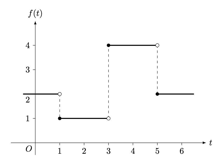
Question 2. Given the function $f$ defined by

$\displaystyle f(t) = \begin{cases}2, & t < 1, \\ 3, & 1 \leq t < 2, \\ 5, & 2 \leq t < 3, \\ 7 , & t \geq 3,\end{cases}$

evaluate $\displaystyle \mathcal L\left\{ \sqrt{f(\sqrt{t})} \cdot U(t - 5)\right\}$ .

(Click for Solution)

Solution. We first observe that

$\displaystyle \sqrt{ f(\sqrt{t}) } = \begin{cases}\sqrt 2, & \sqrt{t} < 1, \\ \sqrt 3, & 1 \leq \sqrt{t} < 2, \\ \sqrt 5, & 2 \leq \sqrt{t} < 3, \\ \sqrt 7 , & \sqrt{t} \geq 3\end{cases} = \begin{cases}\sqrt 2, & t < 1, \\ \sqrt 3, & 1 \leq t < 4, \\ \sqrt 5, & 4 \leq t < 9, \\ \sqrt 7 , & t \geq 9.\end{cases}$

Therefore,

$\displaystyle \sqrt{ f(\sqrt{t}) } \cdot U(t-5) = 0 + \sqrt{5} \cdot U(t-5) + (\sqrt{7} - \sqrt{5}) \cdot U(t-9).$

Taking Laplace transforms,

$\displaystyle \mathcal L\left\{ \sqrt{ f(\sqrt{t}) } \cdot U(t-5) \right\} = \frac 1s \left( \sqrt 5 e^{-5s} + (\sqrt 7 - \sqrt 5) e^{-9s} \right).$

Question 3. Use Laplace transforms to solve the initial value problem

$\displaystyle \left\{ \begin{aligned} y'' - 2y' + 3y &= t^2 \delta(t - 4), \\ y(0) &= 5, \\ y'(0) &= 6.\end{aligned} \right.$

(Click for Solution)

Solution. Taking Laplace transforms on both sides,

$\mathcal L\{y''\} - 2 \mathcal L\{y'\} + 3 \mathcal L\{y\} = \mathcal L\{t^2 \delta(t-4)\}.$

To evaluate the left-hand side,

$\begin{aligned} \mathcal L\{y''\} &= s^2 Y(s) - sy(0) - y'(0) = s^2 Y(s) - 5s - 6, \\ \mathcal L\{y'\} &= s Y(s) - y(0) = s Y(s) - 5, \\ \mathcal L\{y\} &= Y(s). \end{aligned}$

Therefore, the left-hand side simplifies to

$\begin{aligned} & \mathcal L\{y''\} - 2 \mathcal L\{y'\} + 3 \mathcal L\{y\} \\ &= (s^2 Y(s) - 5s - 6) - 2(s Y(s) - 5) + 3Y(s) \\ &= (s^2 - 2s + 3)Y(s) - 5s +4. \end{aligned}$

To evaluate the right-hand side,

$\begin{aligned} \mathcal L\{t^2 \delta(t-4) \} &= -\frac{\mathrm d}{\mathrm ds} \mathcal L\{t \delta(t-4) \} \\ &= -\frac{\mathrm d}{\mathrm ds} \left( -\frac{\mathrm d}{\mathrm ds} \mathcal L\{ \delta(t-4) \} \right) \\ &= -\frac{\mathrm d}{\mathrm ds} \left( -\frac{\mathrm d}{\mathrm ds} (e^{-4s}) \right) = 16e^{-4s}. \end{aligned}$

Putting it all together,

$(s^2 - 2s + 3)Y(s) - 5s +4 = 16e^{-4s}.$

By algebraic manipulation,

$\begin{aligned} Y(s) &= \frac{16 e^{-4s}}{s^2 - 2s + 3} + \frac{5s-4}{s^2 - 2s + 3} \\ y(t) &= 16 \cdot \mathcal L^{-1}\left\{ e^{-4s} \cdot \frac{1}{s^2 - 2s + 3} \right\} + \mathcal L^{-1} \left\{ \frac{5s-4}{s^2 - 2s + 3} \right\}. \end{aligned}$

It remains to (painfully) compute each of the following inverse Laplace transforms, by observing that $s^2 - 2s + 3 = (s-1)^2 + 2$ .

Define $G(s-1) = (5s-4)/((s-1)^2 + 2)$ so that

$\displaystyle G(s) = \frac{5(s+1)-4}{s^2 + 2} = \frac{5s+1}{s^2 + 2} = 5 \cdot \frac s{s^2+2} + \frac 1{s^2+2}.$

By the shift theorems,

$\begin{aligned}\mathcal L^{-1} \left\{ \frac{5s-4}{s^2 - 2s + 3} \right\} &= \mathcal L^{-1}\{ G(s-1)\} \\ &= e^t g(t) \\ &= e^t \cdot \mathcal L^{-1}\left\{ 5 \cdot \frac s{s^2+2} + \frac 1{s^2+2} \right\} \\ &= e^t \cdot \left(5 \cos (t\sqrt 2) + \frac 1{\sqrt 2} \sin(t \sqrt 2) \right).\end{aligned}$

Similarly, defining $H(s) = 1/(s^2 + 2)$ and $H_1 := H(\cdot - 1)$ so that

$\displaystyle h_1(t) = \mathcal L^{-1}\{ H_1(s)\} = \mathcal L^{-1} \{H(s-1)\} = e^t \cdot h(t) = e^t \cdot \frac{1}{\sqrt 2} \sin(t \sqrt 2),$

we have

$\begin{aligned} \mathcal L^{-1}\left\{ e^{-4s} \cdot \frac{1}{s^2 - 2s + 3} \right\} &= \mathcal L^{-1} \{e^{-4s} H_1(s)\} \\ &= h_1(t-4) \cdot U(t-4) \\ &= \frac 1{\sqrt 2} e^{t-4} \sin((t-4)\sqrt 2) \cdot U(t-4). \end{aligned}$

Piecing them all together,

$\displaystyle y(t) = 8\sqrt 2 \cdot e^{t-4} \sin((t-4)\sqrt 2) \cdot U(t-4) + e^t \cdot \left(5 \cos (t\sqrt 2) + \frac 1{\sqrt 2} \sin(t \sqrt 2) \right).$

Question 4. Evaluate the Fourier series of the function $f$ defined by

$f(t) = \begin{cases} 1, & -1 \leq t \leq 0, \\ 2t, & 0 \leq t \leq 1, \end{cases}$

and periodic extension $f(t) = f(t+2)$ .

(Click for Solution)

Solution. We need to evaluate each of the Fourier coefficients $a_0, a_n, b_n$ with $T = 2$ . For $a_0$ ,

$\begin{aligned} a_0 = \int_{-1}^1 f(t)\, \mathrm dt &= \int_{-1}^0 1\, \mathrm dt + \int_0^1 2t\, \mathrm dt \\ &= (0 - (-1)) + (1^2 - 0^2) = 2. \end{aligned}$

For $a_n$ , we need to integrate by parts:

$\begin{aligned} a_n &= \int_{-1}^1 f(t) \cos(n \pi t) \, \mathrm dt \\ &= \int_{-1}^0 \cos(n \pi t)\, \mathrm dt + \int_0^1 2t \cos(n \pi t)\, \mathrm dt \\ &= \left[ \frac{\sin(n \pi t)}{n \pi} \right]_{-1}^0 + \left[ \frac{2 t \sin(n \pi t)}{n \pi} \right]_0^1 + \left[ \frac{2\cos(n \pi t)}{n^2 \pi^2} \right]_0^1 \\ &= 0 + 0 + \frac 2{n^2 \pi^2} ((-1)^n - 1) \\ &= \frac {2 ((-1)^n - 1) }{n^2 \pi^2} . \end{aligned}$

Similarly for $b_n$ , we need to integrate by parts:

$\begin{aligned} b_n &= \int_{-1}^1 f(t) \sin(n \pi t) \, \mathrm dt \\ &= \int_{-1}^0 \sin(n \pi t)\, \mathrm dt + \int_0^1 2t \sin(n \pi t)\, \mathrm dt \\ &= \left[ \frac{-\cos(n \pi t)}{n \pi} \right]_{-1}^0 + \left[ \frac{-2 t \cos(n \pi t)}{n \pi} \right]_0^1 + \left[ \frac{2\sin(n \pi t)}{n^2 \pi^2} \right]_0^1 \\ &= -\frac 1{n\pi} (1 - (-1)^n) - \frac 2{n \pi} (-1)^n \\ &= -\frac 1{n\pi} ( (-1)^n + 1). \end{aligned}$

Therefore, the Fourier series of $f$ is given by

$\displaystyle f(t) = 1 + \sum_{n=1}^\infty \left( \frac {2 ((-1)^n - 1) }{n^2 \pi^2} \cos(n \pi t) -\frac 1{n\pi} ( (-1)^n + 1) \sin(n \pi t) \right).$

—Joel Kindiak, 19 Aug 25, 1613H

August 19, 2025
End-Term Rally

Question 1. Solve the differential equation

$\displaystyle \frac{\mathrm dy}{\mathrm dx} - y = e^{2x}.$

(Click for Solution)

Solution. We identify $P(x) = -1, Q(x) = e^{2x}$ and compute the integrating factor

$I(x) = e^{\int P(x)\, \mathrm dx} = e^{\int -1\, \mathrm dx} = e^{-x}.$

It follows that the general solution is given by

$\begin{aligned} I(x) \cdot y &= \int I(x) Q(x)\, \mathrm dx \\ e^{-x} y &= \int e^{-x} \cdot e^{2x}\, \mathrm dx \\ &= \int e^x \, \mathrm dx \\ &= e^x + C.\end{aligned}$

Question 2. Solve the differential equation

$\displaystyle \frac{\mathrm d^2 y}{\mathrm dx^2} + y = e^{x} \sin(2x).$

(Click for Solution)

Solution. We rewrite the differential equation using $\mathcal D$ -notation:

$(\mathcal D^2 + 1)y = e^x \sin(2x).$

The general solution is given by $y = y_{\mathrm P} + y_{\mathrm C}$ . To compute the complementary function $y_{\mathrm C}$ , we solve $(\mathcal D^2 + 1)y = 0$ . Since the characteristic equation $m^2 + 1 = 0$ has complex conjugate roots $m = \pm i$ , the general solution is given by

$y_{\mathrm C} = C_1 \sin(x) + C_2 \cos(x).$

To compute the particular integral $y_{\mathrm P}$ , we use inverse- $\mathcal D$ notation to evaluate

$\begin{aligned} y_{\mathrm P} &= \frac 1{\mathcal D^2 + 1}(e^x \sin(2x)) \\ &= e^x \cdot \frac 1{(\mathcal D+1)^2 + 1}(\sin(2x)) \\ &= e^x \cdot \frac 1{\mathcal D^2 + 2\mathcal D + 1 + 1}(\sin(2x)) \\ &= e^x \cdot \frac 1{\mathcal D^2 + 2\mathcal D + 2}(\sin(2x)) \\ &= e^x \cdot \frac 1{-2^2 + 2\mathcal D + 2}(\sin(2x)) \\ &= e^x \cdot \frac 1{2\mathcal D - 2}(\sin(2x)) \\ &= \frac 12 e^x \cdot \frac 1{\mathcal D - 1}(\sin(2x)) \\ &= \frac 12 e^x \cdot \frac {\mathcal D+1}{\mathcal D^2 - 1}(\sin(2x)) \\ &= \frac 12 e^x \cdot \frac {\mathcal D+1}{-2^2 - 1}(\sin(2x)) \\ &= -\frac 1{10} e^x \cdot (\mathcal D+1)(\sin(2x)) \\ &= -\frac 1{10} e^x \cdot (\mathcal D(\sin(2x))+\sin(2x)) \\ &= -\frac 1{10} e^x \cdot (2 \cos(2x) +\sin(2x)). \end{aligned}$

Therefore, the general solution is given by

$y = y_{\mathrm P} + y_{\mathrm C} = -\frac 1{10} e^x \cdot (2 \cos(2x) +\sin(2x)) + C_1 \sin(x) + C_2 \cos(x).$

Question 3. Solve the initial value problem

$\displaystyle \left\{ \begin{aligned} y'' + 2y' + 2y &= t^2 \delta(t-2), \\ y(0) &= 0, \\ y'(0) &= 0.\end{aligned} \right.$

(Click for Solution)

Solution. Denote $Y(s) \equiv Y = \mathcal L\{y\} \equiv \mathcal L\{ y(t) \}$ . Taking Laplace transforms on both sides and applying linearity,

$\mathcal L \{y''\} + 2 \cdot \mathcal L\{ y' \} + 2 \cdot \mathcal L \{ y \} = \mathcal L \{ t^2 \delta(t-2) \}.$

Evaluating each of the Laplace transforms,

$\begin{aligned} \mathcal L\{y''\} &= s^2 Y(s) - sy(0) - y'(0) = s^2 Y(s), \\ \mathcal L\{y' \} &= sY(s) - y(0) = sY(s), \\ \mathcal L \{t^2 \delta(t-2) \} &= -\frac{\mathrm d}{\mathrm ds} \mathcal L \{t \delta(t-2)\} \\ &= -\frac{\mathrm d}{\mathrm ds} \left(-\frac{\mathrm d}{\mathrm ds}\mathcal L\{\delta(t-2)\}\right) \\ &= -\frac{\mathrm d}{\mathrm ds} \left(-\frac{\mathrm d}{\mathrm ds} (e^{-2s})\right) \\ &= -\frac{\mathrm d}{\mathrm ds} (2e^{-2s}) \\ &= -(2 \cdot -2e^{-2s}) \\ &= 4e^{-2s}. \end{aligned}$

Substituting all terms,

$\begin{aligned} s^2Y(s) +2s Y(s) + 2Y(s) &= 4e^{-2s} \\ (s^2 + 2s + 2) Y(s) &= 4e^{-2s} \\ Y(s) &= \frac{4 e^{-2s}}{s^2 + 2s + 2}. \end{aligned}$

Motivated by the shift theorems, define $F(s) = 4/(s^2+2s+2)$ . Then

$\begin{aligned} \mathcal L^{-1} \left\{ \frac{4e^{-2s}}{s^2 + 2s + 2} \right\} &= \mathcal L^{-1} \left\{ e^{-2s} F(s) \right\} = f(t-2) U(t-2). \end{aligned}$

It remains to evaluate $f(t) = \mathcal L^{-1} \{F(s)\}$ , which is a nontrivial task. However, if we complete the square on the denominator,

$\displaystyle \frac 4{s^2 + 2s + 2} = \frac 4{(s^2 + 2s + 1) + 1} = \frac 4{(s+1)^2 + 1^2},$

then

$\begin{aligned} f(t) = \mathcal L^{-1} \{F(s)\} &= \mathcal L^{-1} \left\{ \frac 4{(s+1)^2 + 1^2} \right\} = 4 \cdot \mathcal L^{-1} \left\{ \frac 1{(s+1)^2 + 1^2} \right\}. \end{aligned}$

Motivated by the shift theorem again, we define $G(s+1) = 1/((s+1)^2 + 1^2)$ . Then

$f(t) = 4 \cdot \mathcal L^{-1}\{ G(s+1) \} = 4 \cdot e^{-t} g(t),$

where

$\begin{aligned} g(t) = \mathcal L^{-1}\{ G(s) \} &= \mathcal L^{-1} \left\{ \frac 1{s^2 + 1^2} \right\} = \sin(t), \end{aligned}$

so that $f(t) = 4e^{-t} \sin(t)$ . Replacing $t$ with $t-2$ yields the final answer

$\displaystyle \begin{aligned} \mathcal L^{-1} \left\{ \frac{4e^{-2s}}{s^2 + 2s + 2} \right\} &= f(t-2) U(t-2) \\ &= 4 e^{-(t-2)} \sin(t-2) \cdot U(t-2). \end{aligned}$

Question 4. The function $f(t)$ is defined by $f(t) = t^2 + t$ for $-1 \leq t < 1$ and periodic extension $f(t) = f(t+2)$ . Use the Fourier series of $f(t)$ to evaluate the infinite series

$\displaystyle \frac 1{1^2} - \frac 1{2^2} + \frac 1{3^2} - \frac 1{4^2} + \cdots.$

(Click for Solution)

Solution. We contextualise the Fourier series to $T = 2$ :

$\displaystyle f(t) = \frac{a_0}{2} + \sum_{n=1}^\infty \left(a_n \cos (\pi n t) + b_n \sin (\pi n t) \right),$

where

$\displaystyle a_n = \int_{-1}^1 f(t) \cos (\pi n t)\, \mathrm dt,\quad b_n = \int_{-1}^1 f(t) \sin (\pi n t)\, \mathrm dt.$

For $a_n$ , since $\cos(\cdot)$ is even,

$\begin{aligned} a_n &= \int_{-1}^1 f(t) \cos (\pi n t)\, \mathrm dt \\ &= \int_{-1}^1 (t^2 + t) \cos (\pi n t) \, \mathrm dt \\ &= \int_{-1}^1 t^2\cos (\pi n t) \, \mathrm dt + \int_{-1}^1 t \cos (\pi n t) \, \mathrm dt \\ &= 2\int_0^1 t^2\cos (\pi n t) \, \mathrm dt. \end{aligned}$

Similarly, since $\sin(\cdot)$ is odd, we integrate by parts to obtain

$\displaystyle \begin{aligned} b_n &= 2 \int_0^1 t \sin (\pi n t) \, \mathrm dt \\ &= 2 \cdot \left[ t \cdot \frac{-\cos(\pi n t)}{\pi n} + \frac{\sin(\pi n t)}{\pi^2 n^2} \right]_0^1 \\ &= 2 \left( - \frac{\cos(\pi n)}{\pi n}\right) = \frac{2(-1)^{n+1}}{\pi n}. \end{aligned}$

To evaluate $a_n$ for $n \neq 0$ , we integrate by parts to obtain

$\displaystyle \begin{aligned} a_n &= 2 \left( \left[ t^2 \cdot \frac{\sin (\pi n t)}{\pi n} \right]_0^1 - \frac 1{\pi n} \cdot 2 \int_0^1 t \sin(\pi n t)\, \mathrm dt \right) \\ &= 2\left( (0 - 0) -\frac 1{\pi n} \cdot b_n \right) = \frac {4(-1)^n}{\pi^2 n^2}.\end{aligned}$

For the case $n = 0$ ,

$\displaystyle a_0 = 2 \cdot \int_0^1 t^2\, \mathrm dt = 2 \cdot \left[ \frac{t^3}{3} \right]_0^1 = \frac 23.$

Substituting the values of $a_n$ and $b_n$ , the Fourier series of $f(t)$ is given by

$\displaystyle f(t) = \frac 13 - \sum_{n=1}^\infty \left(\frac {4(-1)^{n-1}}{\pi^2 n^2} \cos(\pi n t) - \frac{2(-1)^{n-1}}{\pi n} \sin(\pi n t) \right).$

Setting $t = 0$ , since $f(0) = 0$ ,

$\begin{aligned}0 &= \frac 13 - \frac 4{\pi^2} \sum_{n=1}^\infty \frac {(-1)^{n-1}}{n^2}. \end{aligned}$

By algebruh,

$\displaystyle \frac 1{1^2} - \frac 1{2^2} + \frac 1{3^2} - \frac 1{4^2} + \cdots = \sum_{n=1}^\infty \frac {(-1)^{n-1}}{n^2} = \frac{\pi^2}{12}.$

Remark. If we have $\displaystyle \sum_{n=1}^\infty \frac 1{n^2} = \frac{\pi^2}{6}$ , then

$\displaystyle \begin{aligned} \sum_{n=1}^\infty \frac 1{n^2} - \sum_{n=1}^\infty \frac {(-1)^{n-1}}{n^2} &= \sum_{n=1}^\infty \frac {1- (-1)^{n-1}}{n^2} = \sum_{n=1}^\infty \frac {2}{(2n)^2} = \frac 12 \sum_{n=1}^\infty \frac {1}{n^2}. \end{aligned}$

Then

$\displaystyle \sum_{n=1}^\infty \frac {(-1)^{n-1}}{n^2} = \frac 12 \sum_{n=1}^\infty \frac {1}{n^2} = \frac 12 \cdot \frac{\pi^2}{6} = \frac{\pi^2}{12}.$

—Joel Kindiak, 19 Apr 25, 2352H

August 3, 2025
Infinite Addition

Big Idea

We can approximate any continuous $T$ -periodic function (that is differentiable on $(a, a+T)$ for some $a \in \mathbb R$ ) using its Fourier series given by

$\displaystyle f(t) = \frac{a_0}{2} + \sum_{n=1}^\infty a_n \cos\left( \frac{2\pi n t}{T} \right) + b_n \cos\left( \frac{2\pi n t}{T} \right),$

where

$\displaystyle a_n = \frac{2}{T} \int_{-T/2}^{T/2} f(t)\cos\left( \frac{2\pi n t}{T} \right)\, \mathrm dt,\quad \displaystyle b_n = \frac{2}{T} \int_{-T/2}^{T/2} f(t)\sin\left( \frac{2\pi n t}{T} \right)\, \mathrm dt.$

To simplify computations, it helps to exploit the symmetric properties of odd and even functions. Furthermore, we can use Fourier series to compute infinite sums.

A derivation of the Fourier series (and even a proof that it converges) will require us to venture into abstract linear algebra and even advanced real analysis, far beyond the scope of pre-university mathematics.

Questions

Question 1. Given $f(t) = |t|$ for $-2 \leq t \leq 2$ with periodic extension $f(t) = f(t+4)$ , evaluate the Fourier series of $f(t)$ .

(Click for Solution)

Solution. We contextualise the Fourier series to $T = 4$ :

$\displaystyle f(t) = \frac{a_0}{2} + \sum_{n=1}^\infty \left(a_n \cos \left( \frac{\pi n t}{2} \right) + b_n \sin \left( \frac{\pi n t}{2} \right) \right),$

where

$\displaystyle a_n = \frac 12 \int_{-2}^2 f(t) \cos \left( \frac{\pi n t}{2} \right)\, \mathrm dt,\quad b_n = \frac 12 \int_{-2}^2 f(t) \sin \left( \frac{\pi n t}{2} \right)\, \mathrm dt.$

We observe that $f(t) = |t| = |{-t}| = f(-t)$ so that $f$ is even on $[-2, 2]$ . Since $f(\cdot) \sin(\cdot)$ is odd on $[-2, 2]$ , $b_n = 0$ . For the even term, since $f(\cdot) \cos(\cdot)$ is even on $[-2 ,2]$ ,

$\displaystyle a_n = \frac 12 \int_{-2}^2 f(t) \cos \left( \frac{\pi n t}{2} \right)\, \mathrm dt = \int_0^2 t \cos \left( \frac{\pi n t}{2} \right)\, \mathrm dt.$

For the case $n = 0$ ,

$\displaystyle a_0 = \int_0^2 t \cos (0)\, \mathrm dt = \int_0^2 t\, \mathrm dt = \frac 12 \cdot 2 \cdot 2 = 2.$

For the case $n \neq 0$ , we first make the substitutions

$\displaystyle u = (\pi n t)/2 \quad \iff \quad \mathrm dt = \frac 2{\pi n}\, \mathrm du$

so that $u(2) = n \pi$ and

$\displaystyle \begin{aligned} a_n &= \int_0^2 t \cos \left( \frac{\pi n t}{2} \right)\, \mathrm dt \\ &= \frac 2{n \pi} \int_0^{n \pi} u \cos (u) \cdot \frac 2{\pi n}\, \mathrm du \\ &= \frac 4{ n^2 \pi^2 } \int_0^{n \pi} u \cos (u) \, \mathrm du. \end{aligned}$

Integrating by parts,

$\displaystyle \begin{aligned} \int u \cos(u)\, \mathrm du &= \underbrace{\sin(u)}_{\mathrm I} \underbrace{u}_{\mathrm S} - \int \underbrace{\sin(u)}_{\mathrm I} \underbrace{1}_{\mathrm D}\, \mathrm du \\ &= u \sin(u) - \int \sin(u)\, \mathrm du\\ &= u \sin(u) - (-\cos(u)) + C \\ &= u \sin(u) + \cos(u) + C. \end{aligned}$

Therefore,

$\begin{aligned} a_n &= \frac 4{ n^2 \pi^2 } \left[u \sin(u) + \cos(u) \right]_0^{n \pi} \\ &= \frac 4{ n^2 \pi^2 } ((0 + \cos(n \pi)) - (0 + 1)) \\ &= \frac 4{ n^2 \pi^2 } ( (-1)^n - 1) \\ &= \begin{cases} -\frac{8}{ n^2 \pi^2 }, & n\ \text{odd}, \\ 0, & n\ \text{even}. \end{cases} \end{aligned}$

Substituting the values of $a_n$ and $b_n$ , the Fourier series of $f(t)$ is given by

$\displaystyle f(t) = 1 - \frac {8}{\pi^2} \sum_{k=1}^\infty \frac{1}{(2k-1)^2} \cos \left( \frac{\pi (2k-1) t}{2} \right).$

Question 2. Given $f(t) = |{ \sin(t) }|$ , use the Fourier series of $f(t)$ to evaluate exactly the infinite sum

$\displaystyle \frac 1{2^2 - 1} + \frac 1{4^2 - 1} + \frac 1{6^2 - 1} + \cdots.$

(Click for Solution)

Solution. We contextualise the Fourier series to $T = \pi$ :

$\displaystyle f(t) = \frac{a_0}{2} + \sum_{n=1}^\infty \left(a_n \cos (2n t) + b_n \sin (2n t) \right),$

where

$\displaystyle a_n = \frac 2{\pi} \int_{-\pi/2}^{\pi/2} f(t) \cos (2nt)\, \mathrm dt,\quad b_n = \frac 2{\pi} \int_{-\pi/2}^{\pi/2} f(t) \sin (2nt)\, \mathrm dt.$

We observe that $f(t) = |{\sin(t)}| = |{\sin(-t)}| = f(-t)$ so that $f$ is even on $[-2, 2]$ . Since $f(\cdot) \sin(\cdot)$ is odd on $[-2, 2]$ , $b_n = 0$ . For the even term, since $f(\cdot) \cos(\cdot)$ is even on $[-2 ,2]$ ,

$\displaystyle a_n = \frac 2{\pi} \int_{-\pi/2}^{\pi/2} f(t) \cos (2nt)\, \mathrm dt = \frac 4{\pi} \int_0^{\pi/2} f(t) \cos (2nt)\, \mathrm dt.$

For the case $n = 0$ ,

$\displaystyle a_0 = \frac 4{\pi} \int_0^{\pi/2} \sin(t)\, \mathrm dt = \frac 4{\pi} \left[-{\cos(t)}\right]_0^{\pi/2} = \frac 4{\pi}(0 - (-1)) = \frac 4{\pi}.$

For the case $n \neq 0$ , we integrate by parts to get

$\displaystyle \begin{aligned} & \int \sin(t) \cos (2nt)\, \mathrm dt \\ &= \underbrace{-\cos(t)}_{\mathrm I} \underbrace{\cos (2nt)}_{\mathrm S} - \int \underbrace{-\cos(t)}_{\mathrm I} \underbrace{-2n \sin (2nt)}_{\mathrm D}\, \mathrm dt \\ &= -\cos(t) \cos(2nt) - 2n \int \cos(t) \sin(2nt)\, \mathrm dt \\ &= -\cos(t) \cos(2nt) - 2n \left( \underbrace{\sin(t)}_{\mathrm I} \underbrace{\sin (2nt)}_{\mathrm S} - \int \underbrace{\sin(t)}_{\mathrm I} \underbrace{2n \cos (2nt)}_{\mathrm D}\, \mathrm dt \right) \\ &= -\cos(t) \cos(2nt) -2n \sin(t) \sin(2nt) + 4n^2 \int \sin(t) \cos (2nt)\, \mathrm dt. \end{aligned}$

By algebruh,

$\displaystyle \int \sin(t) \cos (2nt)\, \mathrm dt = \frac{ \cos(t) \cos(2nt) + 2n \sin(t) \sin(2nt)}{4n^2 - 1} + C$

Therefore,

$\begin{aligned} a_n &= \frac 4{\pi} \left[\frac{ \cos(t) \cos(2nt) + 2n \sin(t) \sin(2nt)}{4n^2 - 1} \right]_0^{\pi/2} \\ &= \frac 4{\pi} \left( 0 - \frac 1{4n^2 - 1}\right) = -\frac{4}{\pi(4n^2 - 1)}. \end{aligned}$

Substituting the values of $a_n$ and $b_n$ , the Fourier series of $f(t)$ is given by

$\displaystyle f(t) = \frac 2{\pi} - \frac{4}{\pi} \sum_{k=1}^\infty \frac{1}{4n^2 - 1} \cos (2nt).$

Setting $t = 0$ on both sides, since $f(0) = 0$ ,

$\displaystyle 0 =\frac 2{\pi} - \frac{4}{\pi} \sum_{k=1}^\infty \frac{1}{4n^2 - 1}.$

By algebruh,

$\displaystyle \frac 1{2^2 - 1} + \frac 1{4^2 - 1} + \frac 1{6^2 - 1} + \cdots = \sum_{k=1}^\infty \frac{1}{4n^2 - 1} = \frac 12 .$

Exercise. Try to obtain the same result without the use of Fourier series using a telescoping sum.

—Joel Kindiak, 19 Apr 25, 2240H

July 27, 2025
Applied Laplace Transforms

Big Idea

The Laplace transform can be used to solve initial value problems since

$\mathcal L\{y'(t)\} = sY(s) - y(0),\quad \mathcal L\{y''(t)\} = s^2Y(s) - sy(0) - y'(0).$

For a derivation of these results, check out this post.

Questions

Question 1. Solve the initial value problem

$\left\{ \begin{aligned}y'' + y &= \delta(t-2), \\ y(0) &= 1, \\ y'(0) &= 1. \end{aligned} \right.$

(Click for Solution)

Solution. Taking Laplace transforms on both sides and applying linearity,

$\mathcal L \{ y'' \} + \mathcal L \{ y \} = \mathcal L \{ \delta(t-2) \}.$

Evaluating each term and denoting $Y \equiv Y(s) = \mathcal L\{y(t) \} \equiv \mathcal L\{y(t)\}$ ,

$\begin{aligned} \mathcal L\{ \delta(t-2) \} &= e^{-2s}, \\ \mathcal L\{ y'' \} &= s^2 Y(s) - sy(0) - y'(0) \\ &= s^2 Y(s) - s - 1. \end{aligned}$

Consolidating,

$\begin{aligned} (s^2 Y(s) - s - 1) + Y(s) &= e^{-2s} \\ (s^2 + 1) Y(s) &= s+1 + e^{-2s} \\Y(s) &= \frac s{s^2 + 1} + \frac 1{s^2 + 1} + e^{-2s} \cdot \frac 1{s^2 + 1}. \end{aligned}$

Taking inverse Laplace transforms and applying linearity,

$\begin{aligned} y(t) = \mathcal L^{-1} \{Y(s) \} &= \mathcal L^{-1} \left\{ \frac s{s^2 + 1^2} \right\} + \mathcal L^{-1} \left\{ \frac 1{s^2 + 1^2} \right\} + \mathcal L^{-1} \left\{ e^{-2s} \cdot \frac 1{s^2 + 1} \right\} \\ &= \cos(t) + \sin(t) + \mathcal L^{-1} \left\{ e^{-2s} \cdot \frac 1{s^2 + 1} \right\}.\end{aligned}$

Denoting $F(s) = 1/(s^2+1)$ yields $f(t) = \mathcal L^{-1} \{F(s)\} = \sin(t)$ . By the shift theorems,

$\begin{aligned} \mathcal L^{-1} \{ e^{-2s} F(s) \} &= f(t-2) U (t-2) \\ &= \sin(t-2) U(t-2).\end{aligned}$

Consolidating, we obtain the final answer

$y(t) = \cos(t) + \sin(t) + \sin(t-2) U(t-2).$

Question 2. Solve the initial value problem

$\left\{ \begin{aligned}y'' + y &= 1 + U(t-2), \\ y(0) &= 1, \\ y'(0) &= 1. \end{aligned} \right.$

(Click for Solution)

Solution. Taking Laplace transforms on both sides and applying linearity,

$\mathcal L \{ y'' \} + \mathcal L \{ y \} = \mathcal L\{1\} + \mathcal L \{ U(t-2) \}.$

Evaluating each term and denoting $Y \equiv Y(s) = \mathcal L\{y(t) \} \equiv \mathcal L\{y(t)\}$ ,

$\begin{aligned} \mathcal L\{1\} &= \frac 1s, \\ \mathcal L\{ U(t-2) \} &= \frac{ e^{-2s} }s, \\ \mathcal L\{ y'' \} &= s^2 Y(s) - sy(0) - y'(0) \\ &= s^2 Y(s) - s - 1. \end{aligned}$

Consolidating,

$\begin{aligned} (s^2 Y(s) - s - 1) + Y(s) &= \frac 1s + \frac{ e^{-2s} }s\\ (s^2 + 1) Y(s) &= s+1 + \frac 1s + \frac{ e^{-2s} }s \\Y(s) &= \frac s{s^2 + 1} + \frac 1{s^2 + 1} + \frac 1{s(s^2 + 1)} + e^{-2s} \cdot \frac 1{s( s^2 + 1)} \\ &= \frac {s^2}{s(s^2 + 1)} + \frac 1{s(s^2 + 1)} + \frac 1{s^2 + 1} + e^{-2s} \cdot \frac 1{s( s^2 + 1)} \\ &= \frac {s^2+1}{s(s^2 + 1)} + \frac 1{s^2 + 1} + e^{-2s} \cdot \frac 1{s( s^2 + 1)} \\ &= \frac {1}{s} + \frac 1{s^2 + 1} + e^{-2s} \cdot \frac 1{s( s^2 + 1)}. \end{aligned}$

Taking inverse Laplace transforms and applying linearity,

$\begin{aligned} y(t) = \mathcal L^{-1} \{Y(s) \} &= \mathcal L^{-1} \left\{ \frac 1{s} \right\} + \mathcal L^{-1} \left\{ \frac {1}{s^2 + 1^2} \right\} + \mathcal L^{-1} \left\{ e^{-2s} \cdot \frac 1{s(s^2 + 1)} \right\} \\ &= 1 + \sin(t) + \mathcal L^{-1} \left\{ e^{-2s} \cdot \frac 1{s(s^2 + 1)} \right\}.\end{aligned}$

Denoting $F(s) = 1/(s(s^2+1))$ and performing partial fraction decomposition,

$\displaystyle F(s) = \frac 1{s(s^2 + 1)} = \frac{1}{s} - \frac s{s^2+1}.$

Therefore, $f(t) = \mathcal L^{-1} \{F(s)\} = 1 - \cos(t)$ . By the shift theorems,

$\begin{aligned} \mathcal L^{-1} \{ e^{-2s} F(s) \} &= f(t-2) U (t-2) \\ &= (1 - \cos(t-2)) U(t-2).\end{aligned}$

Consolidating, we obtain the final answer

$y(t) = 1 + \sin(t) + (1 - \cos(t-2)) U(t-2).$

July 20, 2025
Laplace Rally

Question 1. Evaluate $\mathcal L\{1 - t^3 + e^{3t} + \sin(t)\}$ .

(Click for Solution)

Solution. By the linearity of Laplace transforms,

$\begin{aligned} \mathcal L \{1 - t^3 + e^{3t} + \sin(t) \} &= \mathcal L \{ 1\} - \mathcal L \{ t^3 \} + \mathcal L \{ e^{3t} \} + \mathcal L \{ \sin(t) \} \\ &= \frac 1s - \frac{ 3! }{ s^{3+1} } + \frac 1{s-3} + \frac 1{s^2 + 1^2} \\ &= \frac 1s - \frac 6{s^4} + \frac 1{s-3} + \frac 1{s^2+1}. \end{aligned}$

Question 2. Evaluate $\displaystyle \mathcal L^{-1} \left\{ \frac 1{s^2} + \frac 1{s-2} + \frac 1{s^2+9} + \frac s{s^2+4} \right\}$ .

(Click for Solution)

Solution. By the linearity of inverse Laplace transforms,

$\begin{aligned} & \mathcal L^{-1} \left\{ \frac 1{s^2} + \frac 1{s-2} + \frac 1{s^2+9} + \frac s{s^2+4} \right\}\\ &= \mathcal L^{-1} \left\{ \frac{1!}{s^{1+1}} \right\} + \mathcal L^{-1} \left\{ \frac 1{s-2} \right\} \\ &\phantom{==} + \frac 13 \cdot \mathcal L^{-1} \left\{ \frac 3{s^2 + 3^2} \right\} + \mathcal L^{-1} \left\{ \frac s{s^2 + 2^2} \right\} \\ &= t + e^{2t} + \frac 13 \sin(3t)+ \cos(2t). \end{aligned}$

Question 3. The function $f$ is defined by the graph below.

Evaluate $\mathcal L\{e^t f(t)\}$ and $\mathcal L\{f(t) U(t-2)\}$ .

(Click for Solution)

Solution. By observation,

$f(t) = \begin{cases}2, &t < 1, \\ 1, & 1 \leq t < 3, \\ 4, & 3 \leq t < 5, \\ 2, & t \geq 5.\end{cases}$

By the jump technique,

$\begin{aligned} f(t) &= 2 + (1-2) \cdot U(t-1) + (4-1) \cdot U(t-3) + (2-4) \cdot U(t-5) \\ &= 2 - U(t-1) + 3 U(t-3) - 2 U(t-5). \end{aligned}$

By the shift theorems, $\mathcal L\{e^t f(t)\} = F(s-1)$ .

Hence, we need to evaluate $F(s) = \mathcal L\{f(t)\}$ :

$\begin{aligned} F(s) &= \mathcal L\{f(t)\} \\ &= \mathcal L\{ 2 - U(t-1) + 3 U(t-3) - 2 U(t-5) \} \\ &= 2 \cdot \mathcal L\{ 1 \} - \mathcal L \{ U(t-1) \} + 3 \cdot \mathcal L\{ U(t-3) \} - 2 \cdot \mathcal L\{ U(t-5) \} \\ &= 2 \cdot \frac 1{s} - \frac{ e^{-s} }{s} + 3 \cdot \frac{ e^{-3s} }{s} - 2 \cdot \frac{ e^{-5s} }{s} \\ &= \frac 1s (2 - e^{-s} + 3 e^{-3s} - 2 e^{-5s}). \end{aligned}$

Therefore,

$\displaystyle \mathcal L\{e^t f(t)\} = F(s-1) = \frac 1{s-1} (2 - e^{-(s-1)} + 3 e^{-3(s-1)} - 2 e^{-5(s-1)}).$

For the second result, we take advantage of the result

$U(t - a) \cdot U(t - b) = U(t - \max\{a, b\})$

to obtain $f(t) \cdot U(t-2) = U(t-2) + 3 U(t-3) - 2 U(t-5)$ . Taking Laplace transforms,

$\begin{aligned} \mathcal L\{ f(t) \cdot U(t-2) \} &= \frac{e^{-2s}}{s} + 3 \cdot \frac{ e^{-3s} }{s} - 2\cdot \frac{ e^{-5s} }{s} \\ &= \frac 1s (e^{-2s} + 3e^{-3s} - 2e^{-5s}). \end{aligned}$

Question 4. Evaluate $\displaystyle \mathcal L^{-1} \left\{ \frac{4e^{-2s}}{s^2 + 2s + 2} \right\}$ .

(Click for Solution)

Solution. Motivated by the shift theorems, define $F(s) = 4/(s^2+2s+2)$ . Then

$\begin{aligned} \mathcal L^{-1} \left\{ \frac{4e^{-2s}}{s^2 + 2s + 2} \right\} &= \mathcal L^{-1} \left\{ e^{-2s} F(s) \right\} = f(t-2) U(t-2). \end{aligned}$

It remains to evaluate $f(t) = \mathcal L^{-1} \{F(s)\}$ , which is a nontrivial task. However, if we complete the square on the denominator,

$\displaystyle \frac 4{s^2 + 2s + 2} = \frac 4{(s^2 + 2s + 1) + 1} = \frac 4{(s+1)^2 + 1^2},$

then

$\begin{aligned} f(t) = \mathcal L^{-1} \{F(s)\} &= \mathcal L^{-1} \left\{ \frac 4{(s+1)^2 + 1^2} \right\} = 4 \cdot \mathcal L^{-1} \left\{ \frac 1{(s+1)^2 + 1^2} \right\}. \end{aligned}$

Motivated by the shift theorem again, we define $G(s+1) = 1/((s+1)^2 + 1^2)$ . Then

$f(t) = 4 \cdot \mathcal L^{-1}\{ G(s+1) \} = 4 \cdot e^{-t} g(t),$

where

$\begin{aligned} g(t) = \mathcal L^{-1}\{ G(s) \} &= \mathcal L^{-1} \left\{ \frac 1{s^2 + 1^2} \right\} = \sin(t), \end{aligned}$

so that $f(t) = 4e^{-t} \sin(t)$ . Replacing $t$ with $t-2$ yields the final answer

$\displaystyle \begin{aligned} \mathcal L^{-1} \left\{ \frac{4e^{-2s}}{s^2 + 2s + 2} \right\} &= f(t-2) U(t-2) \\ &= 4 e^{-(t-2)} \sin(t-2) \cdot U(t-2). \end{aligned}$

—Joel Kindiak, 19 Apr 25, 1859H

July 6, 2025
Substitutions…Again!

Big Idea

The exponential function in the construction of the Laplace transform yields the dual shift theorems:

$\begin{aligned} \mathcal L\{e^{at}f(t) \} &= F(s-a), \\ \mathcal L^{-1} \{ e^{-as}F(s) \} &= f(t-a)U(t-a). \end{aligned}$

Questions

Question 1. Evaluate $\mathcal L\{te^{2t} + 2e^{3t} - 4e^{2t}\cos(2t)\}$ .

(Click for Solution)

Solution. Factorising $e^{2t}$ ,

$\begin{aligned} te^{2t} + 2e^{3t} - 4e^{2t}\cos(2t) &= e^{2t}\cdot \underbrace{(t + 2e^{t} - 4\cos(2t))}_{f(t)}. \end{aligned}$

By the shift theorems, $\mathcal L\{ e^{2t} f(t) \} = F(s-2)$ . It suffices to evaluate $F(s) = \mathcal L\{f(t)\}$ . By the linearity of Laplace transforms,

$\begin{aligned} F(s) &= \mathcal L\{ t + 2e^{t} - 4\cos(2t) \} \\ &= \mathcal L\{ t \} + 2 \cdot \mathcal L\{ e^t \} - 4 \cdot \mathcal L\{ \cos(2t) \} \\ &= \frac{1!}{s^{1+1}} + 2 \cdot \frac 1{s-1} - 4 \cdot \frac{s}{s^2 + 2^2} \\ &= \frac 1{s^2} + \frac 2{s-1} - \frac{4s}{s^2 + 4}. \end{aligned}$

Hence,

$\displaystyle \begin{aligned} \mathcal L\{e^{2t} f(t)\} &= \frac 1{(s-2)^2} + \frac 2{(s-2)-1} - \frac{4(s-2)}{(s-2)^2 + 4} \\ &= \frac 1{(s-2)^2} + \frac 2{s-3} - \frac{4s-8}{(s-2)^2 + 4}. \end{aligned}$

Question 2. Evaluate $\displaystyle \mathcal L^{-1}\left\{\frac 1{{(s-1)}^3} - \frac 1{s^2 - 2s + 5} + \frac{s-1}{s^2 -2s + 10}\right\}$ .

(Click for Solution)

Solution. Motivated by the first term $1/(s-1)^3$ , define

$\displaystyle F(s-1) := \frac 1{{(s-1)}^3} - \frac 1{s^2 - 2s + 5} + \frac{s-1}{s^2 -2s + 10}.$

Replacing $s$ with $s+1$ in each term,

$\begin{aligned} \frac 1{{(s+1-1)}^3} &= \frac 1{s^3}, \\ \frac 1{(s+1)^2 - 2(s+1) + 5} &= \frac{1}{(s^2 + 2s + 1) - (2s + 2) + 5} = \frac{1}{s^2 + 4}, \\ \frac{(s+1)-1}{(s+1)^2 -2(s+1) + 10} &= \frac{s}{(s^2 + 2s + 1) - (2s + 2) + 10} = \frac{s}{s^2 + 9}. \end{aligned}$

Hence, $\displaystyle F(s) = \frac 1{s^3} - \frac{1}{s^2 + 4} + \frac{s}{s^2 + 9}$ . By the shift theorems,

$\mathcal L^{-1} \{F(s-1)\} = e^{t} f(t).$

It remains to evaluate $f(t) = \mathcal L^{-1}(F(s))$ :

$\begin{aligned} f(t) = \mathcal L^{-1}(F(s)) &= \mathcal L^{-1} \left\{ \frac 1{s^3} - \frac{1}{s^2 + 4} + \frac{s}{s^2 + 9} \right\} \\ &= \mathcal L^{-1} \left\{ \frac 12 \cdot \frac {2!}{s^{2+1}} - \frac 12 \cdot \frac{2}{s^2 + 2^2} + \frac{s}{s^2 + 3^2} \right\} \\ &= \frac 12 t^2 - \frac 12 \sin(2t) + \cos(3t). \end{aligned}$

Therefore, $\mathcal L\{F(s-1)\} = \frac 12 e^{t} (t^2 - \sin(2t) + 2\cos(3t))$ .

Question 3. Evaluate $\mathcal L\{(t-1 + e^{t-2}) \cdot U(t-2)\}$ .

(Click for Solution)

Solution. Motivated by the term $U(t-2)$ , define

$f(t-2) := t-1 + e^{t-2}.$

By the shift theorems,

$\mathcal L\{ f(t-2) U(t-2) \} = e^{-2s} F(s).$

Replacing $t$ with $t+2$ ,

$f(t) = f((t+2) - 2) = (t+2)-1 + e^{(t+2)-2} = t + 1 + e^t.$

Taking Laplace transforms,

$\begin{aligned} F(s) = \mathcal L\{ f(t) \} &= \mathcal L\{ t + 1 + e^t \} \\ &= \frac{1!}{s^{1+1}} + \frac 1s + \frac 1{s-1} \\ &= \frac 1{s^2} + \frac 1s + \frac 1{s-1}. \end{aligned}$

Hence,

$\displaystyle \mathcal L\{ f(t-2) U(t-2) \} = e^{-2s} F(s) = e^{-2s} \cdot \left( \frac 1{s^2} + \frac 1s + \frac 1{s-1} \right).$

Question 4. Evaluate $\displaystyle \mathcal L^{-1} \left\{e^{-3s} \left( \frac 6{s^2+9} -\frac {s+2}{s(s-2)} \right)\right\}$ .

(Click for Solution)

Solution. Define $\displaystyle F(s) = \frac 6{s^2+9} -\frac {s+2}{s(s-2)}$ . By the shift theorems,

$\mathcal L^{-1} \{ e^{-3s} F(s) \} = f(t-3) U(t-3).$

Simplifying $F(s)$ using partial fractions,

$\begin{aligned} F(s) &= \frac 6{s^2+9} -\frac {s+2}{s(s-2)} = \frac 6{s^2+9} + \frac 1s - \frac 2{s-2}. \end{aligned}$

Taking inverse Laplace transforms,

$\begin{aligned} f(t) = \mathcal L^{-1}\{ F(s)\} &= \mathcal L^{-1} \left\{ 2 \cdot \frac 3{s^2+ 3^2} + \frac 1s - 2 \cdot \frac 1{s-2} \right\} \\ &= 2 \sin(3t) + 1 - 2e^{2t}. \end{aligned}$

Therefore,

$\begin{aligned} \mathcal L^{-1} \{ e^{-3s} F(s) \} &= f(t-3) U(t-3) \\ &= (2 \sin(3(t-3)) + 1 - 2e^{2(t-3)}) \cdot U(t-3).\end{aligned}$

—Joel Kindiak, 19 Apr 25, 0107H

June 29, 2025
The Jump Strategy

Big Idea

We can express any finitely-changing step function $f(t)$ in terms of unit-step functions using the following strategy.

$f(t) = (\text{start}) + (\text{jump}_1) \cdot U(t - t_1) + (\text{jump}_2) \cdot U(t - t_2) + \cdots.$

For a complete derivation, see this post. Computing Laplace transforms becomes trivial since $\mathcal L\{\cdot\}$ is linear and $\mathcal L\{U(t-a)\} = e^{-as}/s$ . Recall that the unit step function is defined by

$U(t-a) := \begin{cases} 0, & t < a, \\ 1, & t \geq a. \end{cases}$

Questions

Question 1. The function $f$ is defined by the graph below.

Evaluate $\mathcal L\{f(t)\}$ and $\mathcal L\{(1+f(t))^2\}$ .

(Click for Solution)

Solution. By observation,

$\begin{aligned} f(t) &= \begin{cases}0, &t < 2, \\ 2, & 2 \leq t < 3, \\ 3, & 3 \leq t < 5, \\ 5, & t \geq 5. \end{cases} \end{aligned}$

By the jump technique,

$\begin{aligned} f(t) &= 0 + (2-0)U(t-2) + (3-2)U(t-3) + (5-3)U(t-5) \\ &= 2U(t-2) + U(t-3) + 2U(t-5). \end{aligned}$

By the linearity of Laplace transforms,

$\begin{aligned} \mathcal L\{f(t)\} &= 2 \cdot \mathcal L \{ U(t-2) \} + \mathcal L \{ U(t-3) \} + 2 \cdot \mathcal L \{ U(t-5) \} \\ &= 2 \cdot \frac{ e^{-2s} }{s} + \frac{ e^{-3s} }{s} + 2 \cdot \frac{ e^{-5s} }{s} \\ &= \frac 1s (e^{-2s} + e^{-3s} + 2 e^{-5s}). \end{aligned}$

By the definition of $f$ ,

$\begin{aligned} (1+f(t))^2 &= \begin{cases}(1+0)^2, &t < 2, \\ (1+2)^2, & 2 \leq t < 3, \\ (1+3)^2, & 3 \leq t < 5, \\ (1+5)^2, & t \geq 5, \end{cases} = \begin{cases} 1, &t < 2, \\ 9 & 2 \leq t < 3, \\ 16, & 3 \leq t < 5, \\ 36, & t \geq 5.\end{cases} \end{aligned}$

By the jump technique,

$\begin{aligned}(1+f(t))^2 &= 1 + (9-1)U(t-2) + (16-9)U(t-3) + (36-16)U(t-5) \\ &= 1 + 8U(t-2) + 7U(t-3) + 20 U(t-5). \end{aligned}$

By the linearity of Laplace transforms,

$\begin{aligned}\mathcal L\{ (1+f(t))^2 \} &= \mathcal L\{ 1 \} + 8 \cdot \mathcal L\{ U(t-2) \} + 7 \cdot \mathcal L\{ U(t-3) \} + 20 \cdot \mathcal L\{ U(t-5) \} \\ &= \frac 1s + 8 \cdot \frac{e^{-2s}}{s} + 7 \cdot \frac{e^{-3s}}{s} + 20 \cdot \frac{e^{-5s}}{s} \\ &= \frac 1s (1 + 8e^{-2s} + 7 e^{-3s} + 20e^{-5s}). \end{aligned}$

Question 2. The function $f$ is defined by the graph below.

Evaluate $\mathcal L\{(f(t))^2\}$ and $\mathcal L\{(f(t))^2 \cdot U(t-4)\}$ .

(Click for Solution)

Solution. By observation,

$f(t) = \begin{cases}0, &t < 1, \\ 1, & 1 \leq t < 3, \\ 4, & 3 \leq t < 6, \\ 2, & t \geq 6.\end{cases}$

By the definition of $f$ ,

$\begin{aligned} (f(t))^2 &= \begin{cases}0^2, &t < 1, \\ 1^2, & 1 \leq t < 3, \\ 4^2, & 3 \leq t < 6, \\ 2^2, & t \geq 6,\end{cases} = \begin{cases}0, &t < 1, \\ 1, & 1 \leq t < 3, \\ 16, & 3 \leq t < 6, \\ 4, & t \geq 6.\end{cases} \end{aligned}$

By the jump technique,

$\begin{aligned}(f(t))^2 &= 0 + (1-0)U(t-1) + (16-1)U(t-3) + (4-16)U(t-6) \\ &= U(t-1) + 15U(t-3) -12U(t-6). \end{aligned}$

By the linearity of Laplace transforms,

$\begin{aligned}\mathcal L\{ (f(t))^2 \} &= \mathcal L\{ U(t-1) \} + 15 \cdot \mathcal L\{ U(t-3) \} - 12 \cdot \mathcal L\{ U(t-6) \} \\ &= \frac{e^{-s}}{s} + 15 \cdot \frac{e^{-3s}}{s} - 12 \cdot \frac{e^{-6s}}{s} \\ &= \frac {1}s ( e^{-s} + 15e^{-3s} - 12 e^{-6s}). \end{aligned}$

Since $U(t-a) \cdot U(t-b) = U(t - \max\{a, b\})$ ,

$\begin{aligned} (f(t))^2 \cdot U(t-4) &= U(t-4) + 15U(t-4) -12U(t-6) \\ &= 16 U(t-4) -12 U(t-6). \end{aligned}$

Hence, by the linearity of Laplace transforms,

$\displaystyle \mathcal L\{(f(t))^2 \cdot U(t-4) \} = \frac 1s (16 e^{-4s} - 12 e^{-6s}).$

Question 3. Using the function $f$ defined in Question 2, evaluate

$\displaystyle \mathcal L\left\{\frac 1{1+f(t)} \cdot U(t-4) \right\}.$

(Click for Solution)

Solution. By the definition of $f$ ,

$\begin{aligned} \frac{1}{1+f(t)} &= \begin{cases} \frac{1}{1+0} , &t < 1, \\ \frac{1}{1+1}, & 1 \leq t < 3, \\ \frac{1}{1+4}, & 3 \leq t < 6, \\ \frac{1}{1+2}, & t \geq 6,\end{cases} = \begin{cases}1, &t < 1/2, \\ 1/2, & 1 \leq t < 3, \\ 1/5, & 3 \leq t < 6, \\ 1/3, & t \geq 6.\end{cases} \end{aligned}$

By the jump technique,

$\begin{aligned} \frac 1{1+f(t)} &= 1 + \left(\frac 12 - 1 \right) \cdot U(t-1) + \left(\frac 15 - \frac 12 \right) \cdot U(t-3) + \left(\frac 13 - \frac 15 \right) \cdot U(t-6) \\ &= 1 - \frac 12 \cdot U(t-1) - \frac 3{10} \cdot U(t-3) + \frac 2{15} \cdot U(t-6). \end{aligned}$

Since $U(t-a) \cdot U(t- 4) = U(t- \max \{a, 4\})$ ,

$\displaystyle \begin{aligned} \frac 1{1+f(t)} \cdot U(t-4) &= U(t- 4) - \frac 12 \cdot U(t- 4) - \frac 3{10} \cdot U(t- 4) + \frac 2{15} \cdot U(t-6) \\ &= \frac 1{5} \cdot U(t- 4) + \frac 2{15} \cdot U(t-6). \end{aligned}$

Taking Laplace transforms,

$\displaystyle \mathcal L \left\{ \frac 1{1+f(t)} \right\} = \frac 1s\left(\frac {e^{-4s}}{5} + \frac {2e^{-6s}}{15}\right).$

—Joel Kindiak, 18 Apr 25, 1558H

June 22, 2025
Mid-Term Rally

Big Idea

Laplace transforms are linear transformations:

$\begin{aligned} \mathcal L\{f(t) + g(t)\} &= \mathcal L\{f(t)\} + \mathcal L\{g(t)\}, \\ \mathcal L\{ c \cdot f(t)\}& = c \cdot \mathcal L\{f(t)\}. \end{aligned}$

Often, we denote $F(s) = \mathcal L\{f(t)\}$ , so that inverse Laplace transforms are linear transformations too:

$\begin{aligned} \mathcal L^{-1} \{F(s) + G(s)\} &= \mathcal L^{-1} \{F(s)\} + \mathcal L^{-1} \{G(s)\} \\ \mathcal L^{-1}\{ c \cdot F(s)\} &= c \cdot \mathcal L^{-1}\{F(s)\}. \end{aligned}$

We will also revise previously-discussed topics.

Questions

Question 1. Evaluate $\mathcal L \{ 2 - e^{2t} + \sin(5t) - t^2\}$ .

(Click for Solution)

Solution. By the linearity of Laplace transforms,

$\begin{aligned} \mathcal L \{ 2 - e^{2t} + \sin(5t) - t^2 \} &= 2 \cdot \mathcal L\{ 1 \} - \mathcal L\{ e^{2t} \} + \mathcal L\{ \sin(5t) \} - \mathcal L\{ s^2 \} \\ &= 2 \cdot \frac 1s - \frac 1{s-2} + \frac{5}{s^2+5^2} - \frac{2!}{s^{2+1}} \\ &= \frac 2s - \frac 1{s-2} + \frac 5{s^2 + 25} - \frac 2{s^3}.\end{aligned}$

Question 2. Evaluate

$\displaystyle \mathcal L^{-1} \left\{ \frac 1{s-3} + \frac{s}{s^2 + 4} + \frac 6{s^4} + \frac 1s \right\}.$

(Click for Solution)

Solution. By the linearity of inverse Laplace transforms,

$\begin{aligned} &\mathcal L^{-1} \left\{ \frac 1{s-3} + \frac{s}{s^2 + 4} + \frac 6{s^4} + \frac 1s \right\} \\ &= \mathcal L^{-1} \left\{ \frac 1{s-3} \right\} + \mathcal L^{-1} \left\{ \frac s{s^2+2^2} \right\} + \mathcal L^{-1} \left\{ \frac{3!}{s^{3+1}} \right\} + \mathcal L^{-1} \left\{ \frac 1s \right\} \\ &= e^{3t} + \cos(2t) + t^3 + 1. \end{aligned}$

Question 3. Use Laplace transforms to evaluate $t^2 * \cos(2t)$ .

Hint. Recall that $\mathcal L\{f * g\} = \mathcal L\{f\} \cdot \mathcal L\{g\}$ .

(Click for Solution)

Solution. Taking the Laplace transform of a convolution,

$\begin{aligned} \mathcal L\{ t^2 * \cos(2t) \} &= \mathcal L\{t^2 \} \cdot \mathcal L\{\cos(2t) \} \\ &= \frac{2!}{s^{2+1}} \cdot \frac{s}{s^2 + 2^2} \\ &= \frac 2{s^3} \cdot \frac{s}{s^2 + 4} \\ &= \frac 2{s^2(s^2 + 4)}. \end{aligned}$

Therefore,

$\begin{aligned} t^2 * \cos(2t) &= \mathcal L^{-1} \left\{ \frac 2{s^2(s^2 + 4)} \right\}. \end{aligned}$

Performing partial fraction decomposition (see Problem 15 in this post for the general technique),

$\begin{aligned} \frac{2}{s^2(s^2+4)} &= \frac 12 \left( \frac{1}{s^2} - \frac{1}{s^2+4} \right) = \frac 12 \cdot \frac {1}{s^2} - \frac 14 \cdot \frac{2}{s^2+4}. \end{aligned}$

By the linearity of inverse Laplace transforms,

$\begin{aligned} t^2 * \cos(2t) &= \mathcal L^{-1} \left\{ \frac 2{s^2(s^2 + 4)} \right\} \\ &= \mathcal L^{-1} \left\{ \frac 12 \cdot \frac 1{s^2} - \frac 14 \cdot \frac{2}{s^2+4} \right\} \\ &= \frac 12 \cdot \mathcal L\left\{ \frac 1{s^2} \right\} - \frac 14 \cdot \mathcal L^{-1} \left\{ \frac{2}{s^2+4} \right\} \\ &= \frac 12 \cdot \mathcal L\left\{ \frac {1!}{s^{1+1}} \right\} - \frac 14 \cdot \mathcal L^{-1} \left\{ \frac{2}{s^2+2^2} \right\} \\ &= \frac 12 t - \frac 14 \sin(2t). \end{aligned}$

Remark. Without Laplace transforms, you will need to integrate by parts to obtain

$\begin{aligned} \int u \cos(2u)\, \mathrm du &= \frac 12 u \sin(2u) + \frac 14 \cos(4u) + C, \\ \int u^2 \cos(2u)\, \mathrm du &= \frac 12 u^2 \sin(2u) + \frac 12 u \cos(2u) - \frac 14 \sin(2u) + C ,\end{aligned}$

then use the definition of convolution to get

$\begin{aligned} t^2 * \cos(2t) &= \int_0^t (t-u)^2 \cos(2u)\, \mathrm du \\ &= t^2 \int_0^t \cos(2u)\, \mathrm du - 2u \int_0^t u\cos(2u)\, \mathrm du + \int_0^t u^2 \cos(2u)\, \mathrm du \\ &= t^2 \cdot \frac 12 \sin(2t) - 2t \cdot \left( \frac 12 t \sin(2t) + \frac 14 \cos(2t) - \frac 14 \right) \\ &\phantom{==} + \left( \frac 12 t^2 \sin(2t) + \frac 12 t \cos(2t) - \frac 14 \sin(2t) \right) \\ &= \frac 12 t - \frac 14 \sin(2t). \end{aligned}$

Question 4. Solve the differential equation

$\displaystyle y'' + 2y' - 3y = 4e^x + 5e^{2x}.$

(Click for Solution)

Solution. Rewriting in $\mathcal D$ -notation,

$(\mathcal D^2 + 2 \mathcal D - 3)y = 4e^x + 5e^{2x}.$

The general solution is given by $y = y_{\mathrm P} + y_{\mathrm C}$ . To obtain the complementary function $y_{\mathrm C}$ , we solve the equation

$(\mathcal D^2 + 2 \mathcal D - 3)y = 0.$

Since the characteristic equation $m^2 + 2m - 3 = 0$ has real and distinct auxiliary roots $m = -3, 1$ , the general solution is given by

$y_{\mathrm C} = C_1 e^{-3x} + C_2 e^x.$

To evaluate $y_{\mathrm P}$ , we first use linearity to compute

$\begin{aligned} y_{\mathrm P} &= \frac{1}{\mathcal D^2 + 2 \mathcal D - 3}(4e^x + 5e^{2x}) \\ &= 4 \cdot \underbrace{\frac{1}{\mathcal D^2 + 2 \mathcal D - 3}(e^x)}_{y_1} +\, 5 \cdot \underbrace{\frac{1}{\mathcal D^2 +2 \mathcal D - 3}(e^{2x})}_{y_2}. \end{aligned}$

To shorten presentation, the general solution is $y = 4y_1 + 5y_2 + y_{\mathrm C}$ . For the simpler term $y_2$ ,

$\displaystyle y_2 = \frac{1}{\mathcal D^2 + 2 \mathcal D - 3}(e^{2x}) = \frac 1{2^2 + 2 \cdot 2 - 3} \cdot e^{2x} = \frac{1}{5} e^{2x}.$

For the challenging term $y_1$ , we first replace each $\mathcal D$ with $\mathcal D + 1$ to obtain

$\begin{aligned} (\mathcal D + 1)^2 + 2 (\mathcal D + 1) - 3 &= (\mathcal D^2 + 2\mathcal D + 1) + (2\mathcal D + 2) - 3\\ &= \mathcal D^2 + 4 \mathcal D = \mathcal D(\mathcal D+4). \end{aligned}$

Therefore,

$\begin{aligned} y_1 = \frac{1}{\mathcal D^2 + 2 \mathcal D - 3}(e^{x}) &= e^{x} \cdot \frac{1}{\mathcal D(\mathcal D+4)} (1) \\ &= e^{x} \cdot \frac 1{\mathcal D}\left(\frac 1{\mathcal D+4} (1)\right) \\ &= e^{x} \cdot \frac 1{\mathcal D}\left( \frac 1{0+4} \cdot 1 \right) \\ &= \frac 14 e^x \cdot \frac 1{\mathcal D}(1) = \frac 14 e^x \cdot x. \end{aligned}$

Consolidating all results,

$y = 4y_1 + 5y_2 + y_{\mathrm C} = x e^x + e^{2x} + (C_1 e^{-3x} + C_2 e^x).$

—Joel Kindiak, 18 Apr 25, 1536H

June 1, 2025
Laplace Multipliers

Problem 1. Evaluate $\mathcal L\{\cos^2 t\}$ .

(Click for Solution)

Solution. Applying trigonometric identities,

$\displaystyle \cos^2 t = \frac 12 + \frac 12\cos 2t.$

Taking Laplace transforms on both sides,

$\begin{aligned} \mathcal L\{ \cos^2 t \} &= \mathcal L\left\{ \frac 12 + \frac 12\cos 2t \right\} \\ &= \frac 12\cdot \mathcal L\{1 \} + \frac 12\cdot \mathcal L \{\cos 2t \} \\ &= \frac 12 \cdot \frac 1s + \frac 12 \cdot \frac s{s^2+2^2} \\ &= \frac 1{2s} + \frac {s}{2(s^2+4)}. \end{aligned}$

The point is that calculating the Laplace transform of products is not obvious. Suppose $f$ is any function with Laplace transform $F = \mathcal L \{f\}$ .

Problem 2. Prove that $\mathcal L\{t f(t)\} = -F'(s)$ .

(Click for Solution)

Solution. We need to return to the definition of Laplace transforms:

$\displaystyle \begin{aligned} \mathcal L\{t f(t)\} &= \int_0^\infty t f(t) e^{-st}\, \mathrm dt. \end{aligned}$

The answer is not obvious, but if we pay close attention, we see that differentiating $e^{-st}$ with respect to $s$ yields $e^{-st} \cdot (-t) = -te^{-st}$ . In more technical notation,

$\displaystyle \frac{\partial}{\partial s} (e^{-st}) = -te^{-st},$

where the partial derivative $\partial$ just means that we will treat $t$ as a constant. This means that

$\displaystyle \begin{aligned} \int_0^\infty t f(t) e^{-st}\, \mathrm dt &= \int_0^\infty f(t) \cdot \frac{\partial}{\partial s} (-e^{-st})\, \mathrm dt \\ &= -\int_0^\infty \frac{\partial}{\partial s} (f(t) e^{-st})\, \mathrm dt. \end{aligned}$

We shall now perform a trick: bringing the derivative out of the integral. We will omit the proof of this result as it falls in a far richer study in measure theory and Lebesgue integration. In any case,

$\displaystyle \begin{aligned} \int_0^\infty t f(t) e^{-st}\, \mathrm dt &= -\int_0^\infty \frac{\partial}{\partial s} (f(t) e^{-st})\, \mathrm dt \\ &= -\frac{\mathrm d}{\mathrm ds} \int_0^\infty f(t) e^{-st}\, \mathrm dt\\ &= -F'(s). \end{aligned}$

Problem 3. For any positive integer $n$ , prove that $\mathcal L\{t^n f(t)\} = (-1)^n F^{(n)}(s)$ .

(Click for Solution)

Solution. Applying Problem 2 many more (i.e. $n$ ) times yields

$\mathcal L\{t^n f(t)\} = (-1)^n F^{(n)}(s).$

If multiplying by $t$ gives differentiation, then intuitively, dividing by $t$ ought to yield integration.

Problem 4. Prove that

$\displaystyle \mathcal L\left\{ \frac{f(t)}{t} \right\} = \int_s^\infty F(u)\, \mathrm du,$

assuming that the left-hand side exists.

(Click for Solution)

Solution. We shall return to the definition of Laplace transforms:

$\displaystyle \begin{aligned} \mathcal L\left\{ \frac{f(t)}{t} \right\} &= \int_0^\infty \frac{f(t)}{t} e^{-st}\, \mathrm dt. \end{aligned}$

Similar to Problem 2, if we pay close attention, we see that integrating $e^{-ut}$ with respect to $u$ yields

$\displaystyle \int_s^\infty e^{-ut}\, \mathrm du = \left[ \frac{e^{-ut}}{-t} \right]_s^\infty = 0 - \frac{e^{-st}}{-t} = \frac{e^{-st}}{t}.$

Hence,

$\displaystyle \begin{aligned} \mathcal L\left\{ \frac{f(t)}{t} \right\} &= \int_0^\infty f(t)\int_s^\infty e^{-ut}\, \mathrm du\, \mathrm dt \\ &= \int_0^\infty \int_s^\infty f(t) e^{-ut}\, \mathrm du\, \mathrm dt. \end{aligned}$

We need another tool from multivariable calculus known as Fubini’s theorem, which we will not prove this result in this discussion. This theorem allows us to swap the order of the integrals:

$\displaystyle \begin{aligned} \mathcal L\left\{ \frac{f(t)}{t} \right\} &= \int_0^\infty f(t)\int_s^\infty e^{-ut}\, \mathrm du\, \mathrm dt \\ &= \int_s^\infty \int_0^\infty f(t) e^{-ut}\, \mathrm dt\, \mathrm du \\ &= \int_s^\infty \mathcal L\{f\}(u)\, \mathrm du = \int_s^\infty F(u)\, \mathrm du. \end{aligned}$

Similarly, taking the Laplace transform of an integral ought to transform it into a quotient.

Problem 5. Prove that

$\displaystyle \mathcal L\left\{ \int_0^t f(u)\,\mathrm du \right\} = \frac{F(s)}{s}.$

(Click for Solution)

Solution. Employing the definition of the Laplace transform and Fubini’s theorem,

$\displaystyle \begin{aligned} \mathcal L\left\{ \int_0^t f(u)\,\mathrm du \right\} &= \int_0^\infty \left(\int_0^t f(u)\,\mathrm du \right) \cdot e^{-st}\, \mathrm dt \\ &= \int_0^\infty \int_0^t f(u) e^{-st}\, \mathrm du\, \mathrm dt \\ &= \int_0^\infty \int_u^\infty f(u) e^{-st}\, \mathrm dt\, \mathrm du \\ &= \int_0^\infty f(u) \int_u^\infty e^{-st}\, \mathrm dt\, \mathrm du \\ &= \int_0^\infty f(u) \left[ \frac{e^{-st}}{-s} \right]_u^\infty\, \mathrm du \\ &= \int_0^\infty f(u) \left( 0 - \frac{e^{-su}}{-s} \right)\, \mathrm du \\ &= \frac 1s \int_0^\infty f(u) e^{-su}\, \mathrm du = \frac 1s \cdot F(s) = \frac{F(s)}{s}. \end{aligned}$

Finally for general multiplication problems, while we cannot in general evaluate the Laplace transform of a product, we have a tool to evaluate the inverse Laplace transform of a product.

Problem 6. Given a function $g$ with Laplace transform $G = \mathcal L\{g\}$ , prove that

$\displaystyle \mathcal L^{-1}\{F(s)G(s)\} = \int_0^t f(t-u)g(u)\, \mathrm du =: (f * g)(t).$

(Click for Solution)

Solution. Expanding the definitions of $F$ and $G$ ,

$\begin{aligned} F(s)G(s) &= \int_0^\infty f(v)e^{-sv}\, \mathrm dv \cdot \int_0^\infty g(u)e^{-su}\, \mathrm dv \\ &= \int_0^\infty \int_0^\infty \left( f(v)g(u)\cdot e^{-s(v+u)}\right) \mathrm dv\, \mathrm du \end{aligned}$

Making the substitution $v = t-u \Rightarrow \mathrm dv =\mathrm dt$ ,

$\begin{aligned} F(s)G(s) &= \int_0^\infty \int_{u}^\infty \left( f(t-u)g(u)\cdot e^{-st} \right) \mathrm dt\, \mathrm du \\ &= \int_0^\infty \int_0^t \left( f(t-u)g(u)\cdot e^{-st} \right) \mathrm du\, \mathrm dt \\ &= \int_0^\infty \left( \int_0^t f(t-u)g(u)\, \mathrm du \right) e^{-st} \, \mathrm dt \\ &= \mathcal L\left\{ \int_0^t f(t-u)g(u)\, \mathrm du \right\}, \end{aligned}$

where we used Fubini’s theorem to swap the limits. Hence,

$\displaystyle \mathcal L^{-1}(F(s)G(s)) = \int_0^t f(t-u)g(u)\, \mathrm du =: (f * g)(t)$ ,

where the right-hand side is known as the convolution of the functions $f$ and $g$ .

—Joel Kindiak, 14 Feb 25, 0918H

May 27, 2025