These problems arise from my actual experience, but numbers have been fudged to protect confidentiality.
Problem 1 (Population Mean). As I taught my classes, I noticed that students are exceedingly taller than I. My height is 160 cm, so I suspect that the average height of students is not 160 cm. By collecting the heights cm of 30 randomly chosen students, I obtained the following data:
Test at the 5% significance level to determine whether my suspicion is justified.
(Click for Solution)
Solution. Let denote the height of a randomly chosen student in cm, and .
We first set up the null and alternative hypotheses:
Denote the population variance by and . Assume holds, so that . Since , by the central limit theorem,
Since is unknown, we need to estimate it using :
Furthermore, we estimate using :
Hence, our calculated test statistic will be
Since , , so that using either a – or a -test would yield similar results. Denote and the significance level .
Using a -table, .
Using a -table, .
Whether we let or , it is true that . Therefore, there is sufficient evidence to reject and conclude that Joel’s suspicion is justified, i.e. the average height of students is larger than cm.
Problem 2 (Confidence Intervals). Keep the scenario as Problem 1 but denote the true population mean by . Use the -test for simplicity. Determine the interval of values that can take such that there is insufficient evidence to reject the null hypothesis at the 5% significance.
(Click for Solution)
Solution. By definition,
We do not reject if and only if . Therefore,
Therefore,
Remark 1. We call this calculated interval the -confidence interval for . Denoting a specific sample , let denote the corresponding computed unbiased estimators for respectively. Then the computed corresponding confidence interval will equal
Hence, different samples would yield different confidence intervals. Since is random, so is . Furthermore, defining , mimicking the computation above yields
Thus, we have the following interpretation of a -confidence interval: the probability that a randomly chosen confidence interval will contain the (deterministic though unknown) population mean is .
Problem 3 (Population Proportion). I went to a nearby café, and noticed that there were more women than men in the café. Out of 50 people present, 32 were women.
I suspect that it is true in general that there were more women than men in Starbucks on average. Test at the 5% significance level to determine whether my suspicion is justified.
(Click for Solution)
Solution. Let be a Bernoulli random variable that represents the gender of a person. Here denotes that the person is a man and denotes that the person is a woman. Denote , which yields the proportion of women in the café.
We first set up the null and alternative hypotheses:
Assume holds, so that . We next estimate using :
Since and , by the central limit theorem,
Hence, our calculated test statistic, the -value, will be as follows:
Using a -table, , which holds. Therefore, there is sufficient evidence to reject and conclude that Joel’s suspicion is justified, i.e. there are more women than men on average.
Problem 4 (Goodness-of-Fit). A total of 750 students took an assessment worth marks. For each , let denote the number of students who scored marks out of 10. We have the following data:
Assuming that scores are continuous, determine at the 5% significance level if the scores can be well-approximated using a normal distribution.
(Click for Solution)
Solution. Let denote the score of a randomly chosen student with and . We first set up the null and alternative hypotheses:
We first estimate and using and respectively. Denoting the scores by , the summary statistics are
Hence,
Now we assume holds, so that . Denoting
we will use the test statistic
which follows a -distribution with degrees of freedom. For a proof for why this distribution works, refer to this document. Using relevant -table look-up values (or a spreadsheet application), we obtain the following values for (rounded to the nearest integer for readability, but whose original value we use in the final computation):
Piecing all of the values together,
Using a -table, , which does not hold. Therefore, there is (woefully) insufficient evidence to reject and we cannot conclude that does not follow a normal distribution.
Problem 5 (Population Variance). Using the data in Problem 4, and assuming that the scores are normally distributed, test at the 5% significance level to determine if the standard deviation of assessment scores is greater than 2.
(Click for Solution)
Solution. We first set up the null and alternative hypotheses:
We use the test statistic :
Using a spreadsheet application, . Therefore, there is sufficient evidence to reject and conclude that , which implies .
Definition 1. A continuous random variable is said to follow an exponential distribution with rate parameter, denoted , if
Suppose .
Problem 1. Prove the following properties:
,
,
,
satisfies the memoryless property.
(Click for Solution)
Solution. The c.d.f. of for is given by
Hence,
For the second result, we use the tail-probability characterisation of the expectation, where the interchange of integrals is valid by Fubini’s theorem:
Hence, for ,
For the variance, we adopt a similar approach:
Therefore,
For the memoryless property,
Problem 2. Suppose is independent to .
Calculate the distribution of .
If , evaluate the p.d.f. of .
(Click for Solution)
Solution. Denoting ,
Hence, . To evaluate the p.d.f. of , we compute the convolution of their individual p.d.f.s:
Definition 2. A continuous random variable is said to follow a gamma distribution with shape parameter and rate parameter, denoted if it has a p.d.f. given by
Problem 3. Prove the following properties:
if , then , ,
if are i.i.d., then ,
if and , then .
(Click for Solution)
Solution. Suppose . By definition of the expectation,
Hence, , and
We prove the second result by induction. Suppose and are independent. To evaluate the p.d.f. of , we compute the convolution of their individual p.d.f.s:
Therefore, . Inductively, if are i.i.d.,
For the final property, denoting ,
Hence, .
Given probability distributions , write if there exists a random variable such that and .
Problem 4. Prove the following properties:
,
,
for i.i.d. , ,
for any fixed , if , then .
(Click for Solution)
Solution. We note that if , since ,
so that . If , then
The last two results are immediate corollaries of Problem 3.
These probability distributions are examples of the exponential family of probability distributions.
Feynman’s trick in differentiating under the integral sign has been creatively wielded to evaluate otherwise intractable integrals. In this exercise, we prove Feynman’s trick and use it to evaluate the seemingly intractable Dirichlet integral
Let be a measure space and be a function such that for each , is measurable.
Problem 1. Suppose the following conditions:
For any , is continuous.
There exists some non-negative integrable such that for any , .
Prove that the map defined by is continuous.
(Click for Solution)
Solution. Fix . For any , since is continuous,
so that pointwise. Furthermore,
so that and are all integrable.
Since is integrable, by Lebesgue’s dominated convergence theorem,
so that is continuous, as required.
Problem 2. Suppose the following conditions:
There exists some such that is integrable.
For each , is differentiable with derivative at denoted by .
There exists some non-negative integrable such that for any , .
Prove that the map defined by is differentiable on and
(Click for Solution)
Solution. We first check that is well-defined. By hypothesis, is well-defined. Fix . By the mean value theorem, there exists between and latex t$ such that
By performing more analysis, is integrable, so that is well-defined.
Now fix . For any , since each is measurable,
is measurable. Furthermore, pointwise. We claim that , since the mean value theorem gives between and such that
By algebruh and the triangle inequality, each is integrable. Hence, by Lebesgue’s dominated convergence theorem,
On the other hand, by bookkeeping
Therefore,
Remark 1. Thanks to Problem 2, our proof that in the study of differential equations becomes a logically correct one.
Problem 3. Use Problem 2 to evaluate .
(Click for Solution)
Solution. Define the function by
that satisfies the hypotheses of Problem 2, and our goal is to evaluate . Applying Problem 2 and integrating by parts,
Integrating and applying the first fundamental theorem of calculus,
Problem 1. Let be i.i.d.. Let denote the permutation
such that . Denoting , evaluate for each .
(Click for Solution)
Solution. Since whenever , we can assume .
We will obtain the distribution of . Fix . Let denote the number of sample points that are less than , which follows a binomial distribution. It follows that , so that
Hence, by recalling the properties of the Beta distribution,
Problem 2. Calculate the average number of rolls of a fair six-sided die that you need to roll in order for the sum of all rolls to be a multiple of .
(Click for Solution)
Solution. Let denote the -th roll and denote the sum of the first rolls. Define the stopping time by
$latex\displaystyle N := \inf_{n \in \mathbb N} \{6 \mid X_n\}.$
We claim that . For any ,
For each ,
which is one of the six possible numbers with equal probability:
Therefore, so that as well.
Problem 3. What is the probability of getting an odd number of heads out of independent flips of a fair coin?
(Click for Solution)
Solution. Let denote the number of heads out of independent flips of a fair coin. Then the required probability is
Using properties involving the binomial coefficient,
Therefore,
In particular,
Since , we must have , as required.
Problem 4. Given , calculate .
(Click for Solution)
Solution. Denoting , we observe that
Therefore, by the tail integral for expectation,
Problem 5. You’re the second-best player in a single-elimination tournament with players. Assume the brackets are randomly seeded, and the better player always wins each match. What is the probability you reach the finals?
(Click for Solution)
Solution. Each tournament will have stages, and at stage , there will be players. In order to reach the final stage, we need to be in a different “bracket” with the best player. At stage , there are two “brackets”, and each bracket has players. Therefore, the required probability is
Problem 6. Consider the sample space and the sequence of random variables with the property that
Assuming that has identical distribution, evaluate .
(Click for Solution)
Solution. Denote . By the law of total probability,
Recall that the quantity was defined inductively using Pascal’s identity
and denotes the number of -subsets of a set of size (i.e. distinct objects).
Problem 1. Prove that .
(Click for Solution)
Solution. Fix a set of distinct objects. There are possible -subsets of items that we can remove from that set. Therefore, every -subset of items left behind is obtained by exactly one corresponding -subset of items removed. Therefore, the number of -subsets (left behind) equals the number of -subsets (removed), yielding
Problem 2. Prove that .
(Click for Solution)
Solution. We can interpret the identity as counting the number of -committeees out of persons, and among the persons, we choose persons in a “core team”. This is the quantity counted by the left-hand side:
On the right-hand side, we count the same quantity differently: first choose the “core team” members, then choose the remaining members out of the remaining persons:
Since both types of counting give the same total,
Problem 3. Prove that .
(Click for Solution)
Solution. Replacing with in Problem 2,
Problem 4. Prove that .
(Click for Solution)
Solution. Using Problems 1 and 3,
Problem 5. Prove that .
(Click for Solution)
Solution. Replacing with in Problem 2,
Problem 6. For any , count the number of -tuples such that
(Click for Solution)
Solution. Consider a row of stars and bars. Let denote the number of stars before the 1st bar, denote the number of stars after the 1st bar and before the 2nd bar, and so on and so forth. Each arrangement of the stars and bars then corresponds to each desired -tuple. Thus, the required number is the number of places to place the bars:
Problem 7. For any , suppose is prime. Count the number of -tuples such that
(Click for Solution)
Solution. Since is prime, we require one of the sums to equal , and the other to equal . If the terms sum to , then there are a total of possible options of . By Problem 6, there are a total of


![\mu (\cdot \cap P) \in [0, \infty),\quad \mu (\cdot \cap N) \in (-\infty, 0] ,\quad P \sqcup N = \Omega.](https://s0.wp.com/latex.php?latex=%5Cmu+%28%5Ccdot+%5Ccap+P%29+%5Cin+%5B0%2C+%5Cinfty%29%2C%5Cquad+%5Cmu+%28%5Ccdot+%5Ccap+N%29+%5Cin+%28-%5Cinfty%2C+0%5D+%2C%5Cquad+P+%5Csqcup+N+%3D+%5COmega.&bg=ffffff&fg=000&s=0&c=20201002)


, and
of
for
and
for
.


 cm of 30 randomly chosen students, I obtained the following data:
 denote the height of a randomly chosen student in cm, and
 ![\mu = \mathbb E[X]](https://s0.wp.com/latex.php?latex=%5Cmu+%3D+%5Cmathbb+E%5BX%5D&bg=ffffff&fg=000&s=0&c=20201002) .
. 
 and
and  . Assume
  holds, so that
  . Since
  , by the central limit theorem,
 :
:
 :
:
 will be
 , so that using either a
  – or a
  -test would yield similar results. Denote
  and the significance level
  .
. .
. .
. or
or  , it is true that
  . Therefore, there is sufficient evidence to reject
  cm.
cm. . Use the
 . Therefore,

 -confidence interval for
  , let
, let  denote the corresponding computed unbiased estimators for
  respectively. Then the computed corresponding confidence interval
  will equal
 is random, so is
  , mimicking the computation above yields
 be a Bernoulli random variable that represents the gender of a person. Here
  denotes that the person is a man and
  denotes that the person is a woman. Denote
 ![p := \mathbb E[\xi]](https://s0.wp.com/latex.php?latex=p+%3A%3D+%5Cmathbb+E%5B%5Cxi%5D&bg=ffffff&fg=000&s=0&c=20201002) , which yields the proportion of women in the café.
, which yields the proportion of women in the café.
 . We next estimate
  using
using  :
:
 and
and  , by the central limit theorem,

 , which holds. Therefore, there is sufficient evidence to reject
  marks. For each
  , let
, let  denote the number of students who scored
  marks out of 10. We have the following data:
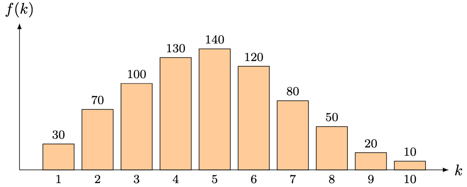
 . We first set up the null and alternative hypotheses:


 . Denoting

 -distribution with
  degrees of freedom. For a proof for why this distribution works, refer to
  (rounded to the nearest integer for readability, but whose original value we use in the final computation):

 , which does not hold. Therefore, there is (woefully) insufficient evidence to reject
 :
:
 . Therefore, there is sufficient evidence to reject
  , which implies
  .
. and
and  , for any
  ,
,
 , if
, if
 ,
,![\mathbb E[X] = 1/\lambda](https://s0.wp.com/latex.php?latex=%5Cmathbb+E%5BX%5D+%3D+1%2F%5Clambda&bg=ffffff&fg=000&s=0&c=20201002) ,
, ,
, of
of  is given by

![\begin{aligned} \mathbb E[X] &= \int_{-\infty}^{\infty} x f_X(x)\, \mathrm dx \\ &= \int_{0}^{\infty} \int_0^x f_X(x)\, \mathrm dy\, \mathrm dx \\ &= \int_{0}^{\infty} \int_{y}^\infty f_X(x) \, \mathrm dx \, \mathrm dy \\ &= \int_{0}^{\infty} \mathbb P(X > y) \, \mathrm dy. \end{aligned}](https://s0.wp.com/latex.php?latex=%5Cbegin%7Baligned%7D+%5Cmathbb+E%5BX%5D+%26%3D+%5Cint_%7B-%5Cinfty%7D%5E%7B%5Cinfty%7D+x+f_X%28x%29%5C%2C+%5Cmathrm+dx+%5C%5C+%26%3D+%5Cint_%7B0%7D%5E%7B%5Cinfty%7D+%5Cint_0%5Ex+f_X%28x%29%5C%2C+%5Cmathrm+dy%5C%2C+%5Cmathrm+dx+%5C%5C+%26%3D+%5Cint_%7B0%7D%5E%7B%5Cinfty%7D+%5Cint_%7By%7D%5E%5Cinfty+f_X%28x%29+%5C%2C+%5Cmathrm+dx+%5C%2C+%5Cmathrm+dy+%5C%5C+%26%3D+%5Cint_%7B0%7D%5E%7B%5Cinfty%7D+%5Cmathbb+P%28X+%3E+y%29+%5C%2C+%5Cmathrm+dy.+%5Cend%7Baligned%7D&bg=ffffff&fg=000&s=0&c=20201002)
![\begin{aligned} \mathbb E[X] &= \int_{0}^{\infty} e^{-\lambda y}\, \mathrm dy = \frac 1{\lambda} \cdot [-e^{-\lambda y}]_0^\infty = \frac 1{\lambda} \cdot (0 - (-1)) = \frac 1{\lambda}. \end{aligned}](https://s0.wp.com/latex.php?latex=%5Cbegin%7Baligned%7D+%5Cmathbb+E%5BX%5D+%26%3D+%5Cint_%7B0%7D%5E%7B%5Cinfty%7D+e%5E%7B-%5Clambda+y%7D%5C%2C+%5Cmathrm+dy+%3D+%5Cfrac+1%7B%5Clambda%7D+%5Ccdot+%5B-e%5E%7B-%5Clambda+y%7D%5D_0%5E%5Cinfty+%3D+%5Cfrac+1%7B%5Clambda%7D+%5Ccdot+%280+-+%28-1%29%29+%3D+%5Cfrac+1%7B%5Clambda%7D.+%5Cend%7Baligned%7D&bg=ffffff&fg=000&s=0&c=20201002)
![\begin{aligned} \mathbb E[X^2] &= \int_{-\infty}^{\infty} 2y \cdot \mathbb P(X > y) \, \mathrm dy \\ &= \int_{0}^{\infty} 2y \cdot e^{-\lambda y} \, \mathrm dy \\ &= \frac 2{\lambda} \int_0^\infty y e^{-\lambda y}\, \mathrm dy \\ &= \frac 2{\lambda} \cdot \mathbb E[X] = \frac 2{\lambda^2}. \end{aligned}](https://s0.wp.com/latex.php?latex=%5Cbegin%7Baligned%7D+%5Cmathbb+E%5BX%5E2%5D+%26%3D+%5Cint_%7B-%5Cinfty%7D%5E%7B%5Cinfty%7D+2y+%5Ccdot+%5Cmathbb+P%28X+%3E+y%29+%5C%2C+%5Cmathrm+dy+%5C%5C+%26%3D+%5Cint_%7B0%7D%5E%7B%5Cinfty%7D+2y+%5Ccdot+e%5E%7B-%5Clambda+y%7D+%5C%2C+%5Cmathrm+dy+%5C%5C+%26%3D+%5Cfrac+2%7B%5Clambda%7D+%5Cint_0%5E%5Cinfty+y+e%5E%7B-%5Clambda+y%7D%5C%2C+%5Cmathrm+dy+%5C%5C+%26%3D+%5Cfrac+2%7B%5Clambda%7D+%5Ccdot+%5Cmathbb+E%5BX%5D+%3D+%5Cfrac+2%7B%5Clambda%5E2%7D.+%5Cend%7Baligned%7D&bg=ffffff&fg=000&s=0&c=20201002)
![\displaystyle \mathrm{Var}(X) = \mathbb E[X^2] - \mathbb E[X]^2 = \frac{2}{\lambda^2} - \frac 1{\lambda^2} = \frac{1}{\lambda^2}.](https://s0.wp.com/latex.php?latex=%5Cdisplaystyle+%5Cmathrm%7BVar%7D%28X%29+%3D+%5Cmathbb+E%5BX%5E2%5D+-+%5Cmathbb+E%5BX%5D%5E2+%3D+%5Cfrac%7B2%7D%7B%5Clambda%5E2%7D+-+%5Cfrac+1%7B%5Clambda%5E2%7D+%3D+%5Cfrac%7B1%7D%7B%5Clambda%5E2%7D.&bg=ffffff&fg=000&s=0&c=20201002)

 is independent to
  .
. , evaluate the p.d.f. of
  .
. ,
,
 . To evaluate the p.d.f. of
  , we compute the convolution of their individual p.d.f.s:
 and rate parameter
  if it has a p.d.f. given by
 , then
 ![\mathbb E[X] = \alpha/\lambda](https://s0.wp.com/latex.php?latex=%5Cmathbb+E%5BX%5D+%3D+%5Calpha%2F%5Clambda&bg=ffffff&fg=000&s=0&c=20201002) ,
,  ,
, are i.i.d., then
  ,
, , then
  .
. . By definition of the expectation,
![\begin{aligned} \mathbb E[X^n] &= \int_0^\infty x^n \cdot \frac{\lambda^\alpha}{\Gamma(\alpha)} \cdot x^{\alpha - 1} \cdot e^{-\lambda x}\, \mathrm dx \\ &= \frac {\alpha \cdot (\alpha+1) \cdot \cdots \cdot (\alpha +n-1)}{\lambda^n} \cdot \int_0^\infty \frac{\lambda^{\alpha+n}}{\Gamma(\alpha+1)} \cdot x^{(\alpha + n) - 1} \cdot e^{-\lambda x}\, \mathrm dx \\ &= \frac{\alpha \cdot (\alpha+1) \cdot \cdots \cdot (\alpha +n-1)}{\lambda^n} \cdot \int_0^\infty f_Y(x)\, \mathrm dx \\ &= \frac{\alpha \cdot (\alpha+1) \cdot \cdots \cdot (\alpha +n-1)}{\lambda^n} . \end{aligned}](https://s0.wp.com/latex.php?latex=%5Cbegin%7Baligned%7D+%5Cmathbb+E%5BX%5En%5D+%26%3D+%5Cint_0%5E%5Cinfty+x%5En+%5Ccdot+%5Cfrac%7B%5Clambda%5E%5Calpha%7D%7B%5CGamma%28%5Calpha%29%7D+%5Ccdot+x%5E%7B%5Calpha+-+1%7D+%5Ccdot+e%5E%7B-%5Clambda+x%7D%5C%2C+%5Cmathrm+dx+%5C%5C+%26%3D+%5Cfrac+%7B%5Calpha+%5Ccdot+%28%5Calpha%2B1%29+%5Ccdot+%5Ccdots+%5Ccdot+%28%5Calpha+%2Bn-1%29%7D%7B%5Clambda%5En%7D+%5Ccdot+%5Cint_0%5E%5Cinfty+%5Cfrac%7B%5Clambda%5E%7B%5Calpha%2Bn%7D%7D%7B%5CGamma%28%5Calpha%2B1%29%7D+%5Ccdot+x%5E%7B%28%5Calpha+%2B+n%29+-+1%7D+%5Ccdot+e%5E%7B-%5Clambda+x%7D%5C%2C+%5Cmathrm+dx+%5C%5C+%26%3D+%5Cfrac%7B%5Calpha+%5Ccdot+%28%5Calpha%2B1%29+%5Ccdot+%5Ccdots+%5Ccdot+%28%5Calpha+%2Bn-1%29%7D%7B%5Clambda%5En%7D+%5Ccdot+%5Cint_0%5E%5Cinfty+f_Y%28x%29%5C%2C+%5Cmathrm+dx+%5C%5C+%26%3D+%5Cfrac%7B%5Calpha+%5Ccdot+%28%5Calpha%2B1%29+%5Ccdot+%5Ccdots+%5Ccdot+%28%5Calpha+%2Bn-1%29%7D%7B%5Clambda%5En%7D+.+%5Cend%7Baligned%7D&bg=ffffff&fg=000&s=0&c=20201002)
![\begin{aligned} \mathrm{Var}(X) &= \mathbb E[X^2] - \mathbb E[X]^2 = \frac{\alpha \cdot (\alpha+1)}{\lambda^2} - \frac{\alpha^2}{\lambda^2} = \frac{\alpha}{\lambda^2}. \end{aligned}](https://s0.wp.com/latex.php?latex=%5Cbegin%7Baligned%7D+%5Cmathrm%7BVar%7D%28X%29+%26%3D+%5Cmathbb+E%5BX%5E2%5D+-+%5Cmathbb+E%5BX%5D%5E2+%3D+%5Cfrac%7B%5Calpha+%5Ccdot+%28%5Calpha%2B1%29%7D%7B%5Clambda%5E2%7D+-+%5Cfrac%7B%5Calpha%5E2%7D%7B%5Clambda%5E2%7D+%3D+%5Cfrac%7B%5Calpha%7D%7B%5Clambda%5E2%7D.+%5Cend%7Baligned%7D&bg=ffffff&fg=000&s=0&c=20201002)
 are independent. To evaluate the p.d.f. of
 . Inductively, if
 ,
,
 .
. , write
  if there exists a random variable
  and
and  .
. ,
, ,
, ,
,  ,
, , then
  .
. , since
  ,
,
 . If
. If  , then
 , a random variable
  satisfies the memoryless property if the following holds: for any
  ,
,
 and
and  in terms of
  .
. by
by  . By the definition of conditional probability,
 for some
  . In particular,
 , so that
 is said to follow a geometric distribution with success probability
  , if
, if


![\displaystyle \mathbb E[X] = \sum_{x = 0}^\infty \mathbb P(X > x)](https://s0.wp.com/latex.php?latex=%5Cdisplaystyle+%5Cmathbb+E%5BX%5D+%3D+%5Csum_%7Bx+%3D+0%7D%5E%5Cinfty+%5Cmathbb+P%28X+%3E+x%29&bg=ffffff&fg=000&s=0&c=20201002) . Hence, evaluate
. Hence, evaluate ![\mathbb E[X]](https://s0.wp.com/latex.php?latex=%5Cmathbb+E%5BX%5D&bg=ffffff&fg=000&s=0&c=20201002) and
and  .
.![\begin{aligned} \mathbb E[X] &= \sum_{x = 0}^\infty x \cdot \mathbb P(X = x) \\ &= \sum_{x=0}^\infty \sum_{y=0}^{x-1} \mathbb P(X = x) \\ &= \sum_{y=0}^\infty \sum_{x=y+1}^\infty \mathbb P(X = x) \\ &= \sum_{y=0}^\infty \mathbb P(X > y) = \sum_{x = 0}^\infty \mathbb P(X > x). \end{aligned}](https://s0.wp.com/latex.php?latex=%5Cbegin%7Baligned%7D+%5Cmathbb+E%5BX%5D+%26%3D+%5Csum_%7Bx+%3D+0%7D%5E%5Cinfty+x+%5Ccdot+%5Cmathbb+P%28X+%3D+x%29+%5C%5C+%26%3D+%5Csum_%7Bx%3D0%7D%5E%5Cinfty+%5Csum_%7By%3D0%7D%5E%7Bx-1%7D+%5Cmathbb+P%28X+%3D+x%29+%5C%5C+%26%3D+%5Csum_%7By%3D0%7D%5E%5Cinfty+%5Csum_%7Bx%3Dy%2B1%7D%5E%5Cinfty+%5Cmathbb+P%28X+%3D+x%29+%5C%5C+%26%3D+%5Csum_%7By%3D0%7D%5E%5Cinfty+%5Cmathbb+P%28X+%3E+y%29+%3D+%5Csum_%7Bx+%3D+0%7D%5E%5Cinfty+%5Cmathbb+P%28X+%3E+x%29.+%5Cend%7Baligned%7D&bg=ffffff&fg=000&s=0&c=20201002)
![\displaystyle \mathbb E[X] = \sum_{x=0}^\infty (1-p)^x = \frac{1}{1-(1-p)} = \frac 1p.](https://s0.wp.com/latex.php?latex=%5Cdisplaystyle+%5Cmathbb+E%5BX%5D+%3D+%5Csum_%7Bx%3D0%7D%5E%5Cinfty+%281-p%29%5Ex+%3D+%5Cfrac%7B1%7D%7B1-%281-p%29%7D+%3D+%5Cfrac+1p.&bg=ffffff&fg=000&s=0&c=20201002)
![\mathbb E[X^2]](https://s0.wp.com/latex.php?latex=%5Cmathbb+E%5BX%5E2%5D&bg=ffffff&fg=000&s=0&c=20201002) . Observe that
. Observe that
![\begin{aligned} \mathbb E[X^2] &= \sum_{x = 0}^\infty x^2 \cdot \mathbb P(X = x) \\ &= \sum_{x=0}^\infty \sum_{y=0}^{x-1} (2y + 1) \cdot \mathbb P(X = x) \\ &= \sum_{y=0}^\infty \sum_{x=y+1}^\infty (2y + 1) \cdot \mathbb P(X = x) \\ &= \sum_{y=0}^\infty \left( (2y + 1) \cdot \sum_{x=y+1}^\infty (1-p)^{x-1} \cdot p \right) \\ &= \sum_{y=0}^\infty \left( (2y + 1) \cdot \frac{(1-p)^y}{1 - (1-p)} \cdot p \right) \\ &= \frac 1p \cdot \sum_{y=0}^\infty \left( (2y + 1) \cdot (1-p)^y \cdot p \right) \\ &= \frac 1p \cdot \left( p + (1-p) \cdot \left( 2 \cdot \sum_{y=1}^\infty y\cdot \mathbb P(X = y ) + \sum_{y=1}^\infty \mathbb P(X = y ) \right) \right) \\ &= \frac 1p \cdot \left( p + (1-p) \cdot \left( \frac 2p + 1 \right) \right) \\ &= 1 + \left( \frac 1p - 1 \right) \cdot \left( \frac 2p + 1 \right) \\ &= 1 + \frac 2{p^2} + \frac 1p - \frac 2p - 1 = \frac {2-p}{p^2}. \end{aligned}](https://s0.wp.com/latex.php?latex=%5Cbegin%7Baligned%7D+%5Cmathbb+E%5BX%5E2%5D+%26%3D+%5Csum_%7Bx+%3D+0%7D%5E%5Cinfty+x%5E2+%5Ccdot+%5Cmathbb+P%28X+%3D+x%29+%5C%5C+%26%3D+%5Csum_%7Bx%3D0%7D%5E%5Cinfty+%5Csum_%7By%3D0%7D%5E%7Bx-1%7D+%282y+%2B+1%29+%5Ccdot+%5Cmathbb+P%28X+%3D+x%29+%5C%5C+%26%3D+%5Csum_%7By%3D0%7D%5E%5Cinfty+%5Csum_%7Bx%3Dy%2B1%7D%5E%5Cinfty+%282y+%2B+1%29+%5Ccdot+%5Cmathbb+P%28X+%3D+x%29+%5C%5C+%26%3D+%5Csum_%7By%3D0%7D%5E%5Cinfty+%5Cleft%28+%282y+%2B+1%29+%5Ccdot+%5Csum_%7Bx%3Dy%2B1%7D%5E%5Cinfty+%281-p%29%5E%7Bx-1%7D+%5Ccdot+p+%5Cright%29+%5C%5C+%26%3D+%5Csum_%7By%3D0%7D%5E%5Cinfty+%5Cleft%28+%282y+%2B+1%29+%5Ccdot+%5Cfrac%7B%281-p%29%5Ey%7D%7B1+-+%281-p%29%7D+%5Ccdot+p+%5Cright%29+%5C%5C+%26%3D+%5Cfrac+1p+%5Ccdot+%5Csum_%7By%3D0%7D%5E%5Cinfty+%5Cleft%28+%282y+%2B+1%29+%5Ccdot+%281-p%29%5Ey+%5Ccdot+p+%5Cright%29+%5C%5C+%26%3D+%5Cfrac+1p+%5Ccdot+%5Cleft%28+p+%2B+%281-p%29+%5Ccdot++%5Cleft%28+2+%5Ccdot+%5Csum_%7By%3D1%7D%5E%5Cinfty+y%5Ccdot+%5Cmathbb+P%28X+%3D+y+%29++%2B+%5Csum_%7By%3D1%7D%5E%5Cinfty+%5Cmathbb+P%28X+%3D+y+%29++%5Cright%29+%5Cright%29+%5C%5C+%26%3D+%5Cfrac+1p+%5Ccdot+%5Cleft%28+p+%2B+%281-p%29+%5Ccdot++%5Cleft%28+%5Cfrac+2p++%2B+1+%5Cright%29+%5Cright%29+%5C%5C+%26%3D+1+%2B+%5Cleft%28+%5Cfrac+1p+-+1+%5Cright%29+%5Ccdot+%5Cleft%28+%5Cfrac+2p++%2B+1+%5Cright%29+%5C%5C+%26%3D+1+%2B+%5Cfrac+2%7Bp%5E2%7D+%2B+%5Cfrac+1p+-+%5Cfrac+2p+-+1+%3D+%5Cfrac+%7B2-p%7D%7Bp%5E2%7D.+%5Cend%7Baligned%7D&bg=ffffff&fg=000&s=0&c=20201002)
![\begin{aligned} \mathrm{Var}(X) &= \mathbb E[X^2] -\mathbb E[X]^2 = \frac {2-p}{p^2} - \frac 1{p^2} = \frac{1-p}{p^2}. \end{aligned}](https://s0.wp.com/latex.php?latex=%5Cbegin%7Baligned%7D+%5Cmathrm%7BVar%7D%28X%29+%26%3D+%5Cmathbb+E%5BX%5E2%5D+-%5Cmathbb+E%5BX%5D%5E2+%3D+%5Cfrac+%7B2-p%7D%7Bp%5E2%7D+-+%5Cfrac+1%7Bp%5E2%7D+%3D+%5Cfrac%7B1-p%7D%7Bp%5E2%7D.+%5Cend%7Baligned%7D&bg=ffffff&fg=000&s=0&c=20201002)
 is independent of
  . Then
 .
. . For any

 .
. is even in

![\begin{aligned}\left( \int_{0}^{\infty} e^{-x^2}\, \mathrm dx \right)^2 &= \int_0^\infty \int_0^\infty xe^{-x^2(u^2+1)} \, \mathrm du\, \mathrm dx\\ &= \int_0^\infty \int_0^\infty xe^{-x^2(u^2+1)} \, \mathrm dx\, \mathrm du \\ &= \int_0^\infty \left[ -\frac 1{2(u^2+1)} \cdot e^{-x^2(u^2+1)} \right]_0^\infty\, \mathrm du \\ &= \int_0^\infty \frac 1{2(u^2+1)}\, \mathrm du \\ &= \frac 12 \cdot [\tan^{-1}(u)]_0^{\infty} \\ &= \frac 12 \cdot \frac{\pi}2 = \frac{\pi}{4}. \end{aligned}](https://s0.wp.com/latex.php?latex=%5Cbegin%7Baligned%7D%5Cleft%28+%5Cint_%7B0%7D%5E%7B%5Cinfty%7D+e%5E%7B-x%5E2%7D%5C%2C+%5Cmathrm+dx+%5Cright%29%5E2+%26%3D+%5Cint_0%5E%5Cinfty+%5Cint_0%5E%5Cinfty+xe%5E%7B-x%5E2%28u%5E2%2B1%29%7D+%5C%2C+%5Cmathrm+du%5C%2C+%5Cmathrm+dx%5C%5C++%26%3D+%5Cint_0%5E%5Cinfty+%5Cint_0%5E%5Cinfty+xe%5E%7B-x%5E2%28u%5E2%2B1%29%7D+%5C%2C+%5Cmathrm+dx%5C%2C+%5Cmathrm+du+%5C%5C+%26%3D+%5Cint_0%5E%5Cinfty+%5Cleft%5B+-%5Cfrac+1%7B2%28u%5E2%2B1%29%7D+%5Ccdot+e%5E%7B-x%5E2%28u%5E2%2B1%29%7D+%5Cright%5D_0%5E%5Cinfty%5C%2C+%5Cmathrm+du+%5C%5C+%26%3D+%5Cint_0%5E%5Cinfty+%5Cfrac+1%7B2%28u%5E2%2B1%29%7D%5C%2C+%5Cmathrm+du+%5C%5C+%26%3D+%5Cfrac+12+%5Ccdot+%5B%5Ctan%5E%7B-1%7D%28u%29%5D_0%5E%7B%5Cinfty%7D+%5C%5C+%26%3D+%5Cfrac+12+%5Ccdot+%5Cfrac%7B%5Cpi%7D2+%3D+%5Cfrac%7B%5Cpi%7D%7B4%7D.+%5Cend%7Baligned%7D&bg=ffffff&fg=000&s=0&c=20201002)

 follows a Poisson distribution with rate parameter
  , if
, if
 .
. .
. :
:
 .
.![\begin{aligned} \mathbb E[X] &= \sum_{x = 0}^\infty x \cdot \mathbb P(X=x) \\ &= \sum_{x = 1}^\infty x \cdot c_\lambda \cdot \frac{\lambda^x}{x!} \\ &= \lambda \cdot \sum_{x = 1}^\infty c_\lambda \cdot \frac{\lambda^{x-1}}{(x-1)!} \\ &= \lambda \cdot \sum_{x = 0}^\infty c_\lambda \cdot \frac{\lambda^{x}}{x!} = \lambda \cdot 1 = \lambda. \end{aligned}](https://s0.wp.com/latex.php?latex=%5Cbegin%7Baligned%7D+%5Cmathbb+E%5BX%5D+%26%3D+%5Csum_%7Bx+%3D+0%7D%5E%5Cinfty+x+%5Ccdot+%5Cmathbb+P%28X%3Dx%29+%5C%5C+%26%3D+%5Csum_%7Bx+%3D+1%7D%5E%5Cinfty+x+%5Ccdot+c_%5Clambda+%5Ccdot+%5Cfrac%7B%5Clambda%5Ex%7D%7Bx%21%7D+%5C%5C+%26%3D+%5Clambda+%5Ccdot+%5Csum_%7Bx+%3D+1%7D%5E%5Cinfty+c_%5Clambda+%5Ccdot+%5Cfrac%7B%5Clambda%5E%7Bx-1%7D%7D%7B%28x-1%29%21%7D+%5C%5C+%26%3D+%5Clambda+%5Ccdot++%5Csum_%7Bx+%3D+0%7D%5E%5Cinfty+c_%5Clambda+%5Ccdot+%5Cfrac%7B%5Clambda%5E%7Bx%7D%7D%7Bx%21%7D+%3D+%5Clambda+%5Ccdot+1+%3D+%5Clambda.+%5Cend%7Baligned%7D&bg=ffffff&fg=000&s=0&c=20201002)
![\begin{aligned}\mathbb E[X(X-1)] &= \sum_{x = 0}^\infty x(x-1) \cdot \mathbb P(X=x) \\ &= \sum_{x = 2}^\infty x(x-1) \cdot c_\lambda \cdot \frac{\lambda^x}{x!} \\ &= \lambda^2 \cdot \sum_{x = 2}^\infty c_\lambda \cdot \frac{\lambda^{x-2}}{(x-2)!} \\ &= \lambda^2 \cdot 1 = \lambda^2. \end{aligned}](https://s0.wp.com/latex.php?latex=%5Cbegin%7Baligned%7D%5Cmathbb+E%5BX%28X-1%29%5D+%26%3D+%5Csum_%7Bx+%3D+0%7D%5E%5Cinfty+x%28x-1%29+%5Ccdot+%5Cmathbb+P%28X%3Dx%29+%5C%5C+%26%3D+%5Csum_%7Bx+%3D+2%7D%5E%5Cinfty+x%28x-1%29+%5Ccdot+c_%5Clambda+%5Ccdot+%5Cfrac%7B%5Clambda%5Ex%7D%7Bx%21%7D+%5C%5C+%26%3D+%5Clambda%5E2+%5Ccdot+%5Csum_%7Bx+%3D+2%7D%5E%5Cinfty+c_%5Clambda+%5Ccdot+%5Cfrac%7B%5Clambda%5E%7Bx-2%7D%7D%7B%28x-2%29%21%7D+%5C%5C+%26%3D+%5Clambda%5E2+%5Ccdot+1+%3D+%5Clambda%5E2.+%5Cend%7Baligned%7D&bg=ffffff&fg=000&s=0&c=20201002)
![\begin{aligned} \mathrm{Var}(X) &= \mathbb E[X^2] - \mathbb E[X]^2 \\ &= \mathbb E[X(X-1)] + \mathbb E[X] - \mathbb E[X]^2 \\ &= \lambda^2 + \lambda - \lambda^2 = \lambda.\end{aligned}](https://s0.wp.com/latex.php?latex=%5Cbegin%7Baligned%7D+%5Cmathrm%7BVar%7D%28X%29+%26%3D+%5Cmathbb+E%5BX%5E2%5D+-+%5Cmathbb+E%5BX%5D%5E2+%5C%5C+%26%3D+%5Cmathbb+E%5BX%28X-1%29%5D+%2B+%5Cmathbb+E%5BX%5D+-+%5Cmathbb+E%5BX%5D%5E2+%5C%5C+%26%3D+%5Clambda%5E2+%2B+%5Clambda+-+%5Clambda%5E2+%3D+%5Clambda.%5Cend%7Baligned%7D&bg=ffffff&fg=000&s=0&c=20201002)
 are independent, determine the distribution of
  , we take the discrete convolution of the p.d.f.s of
  to obtain
 . Hence,
 .
. and
and  . Prove that
  .
. . For each
  ,
,
 ,
,

 be a measure space and
 ![f : \Omega \times [a, b] \to \mathbb R](https://s0.wp.com/latex.php?latex=f+%3A+%5COmega+%5Ctimes+%5Ba%2C+b%5D+%5Cto+%5Cmathbb+R&bg=ffffff&fg=000&s=0&c=20201002) be a function such that for each
be a function such that for each ![t \in [a, b]](https://s0.wp.com/latex.php?latex=t+%5Cin+%5Ba%2C+b%5D&bg=ffffff&fg=000&s=0&c=20201002) ,
,  is measurable.
 ,
,  is continuous.
 such that for any
 ![(\omega, t) \in \Omega \times [a, b]](https://s0.wp.com/latex.php?latex=%28%5Comega%2C+t%29+%5Cin+%5COmega+%5Ctimes+%5Ba%2C+b%5D&bg=ffffff&fg=000&s=0&c=20201002) ,
,  .
.![F : [a, b] \to \mathbb R](https://s0.wp.com/latex.php?latex=F+%3A+%5Ba%2C+b%5D+%5Cto+%5Cmathbb+R&bg=ffffff&fg=000&s=0&c=20201002) defined by
defined by  is continuous.
 . For any
 pointwise. Furthermore,
 and
and  are all integrable.
 is integrable, by Lebesgue’s dominated convergence theorem,
 is continuous, as required.
![t_0 \in [a, b]](https://s0.wp.com/latex.php?latex=t_0+%5Cin+%5Ba%2C+b%5D&bg=ffffff&fg=000&s=0&c=20201002) such that
such that  is integrable.
 denoted by
  .
. .
. is differentiable on
 ![[a, b]](https://s0.wp.com/latex.php?latex=%5Ba%2C+b%5D&bg=ffffff&fg=000&s=0&c=20201002) and
and
 is well-defined. Fix
 is well-defined.
 is measurable,
 pointwise. We claim that
  , since the mean value theorem gives
  and
and 
 is integrable. Hence, by Lebesgue’s dominated convergence theorem,


 in the study of differential equations becomes a logically correct one.
 .
. by
by
 . Applying Problem 2 and integrating by parts,
![\begin{aligned} I'(y) &= \int_{0}^{\infty} \frac{\partial}{\partial y} \left( \frac{\sin x}{x} \cdot e^{-xy} \right) \, \mathrm dx \\ &= \int_{0}^{\infty} \frac{\sin x}{x} \cdot -xe^{-xy} \, \mathrm dx \\ &= -\int_{0}^{\infty} e^{-xy} \cdot \sin x \, \mathrm dx \\ &= -\left[ \frac{e^{-xy}}{(-y)^2 + 1^2} \cdot ((-y) \sin(x) - \cos(x)) \right]_{0}^{\infty} \\ &= -\frac{1}{1+y^2}. \end{aligned}](https://s0.wp.com/latex.php?latex=%5Cbegin%7Baligned%7D+I%27%28y%29+%26%3D+%5Cint_%7B0%7D%5E%7B%5Cinfty%7D+%5Cfrac%7B%5Cpartial%7D%7B%5Cpartial+y%7D+%5Cleft%28+%5Cfrac%7B%5Csin+x%7D%7Bx%7D+%5Ccdot+e%5E%7B-xy%7D+%5Cright%29+%5C%2C+%5Cmathrm+dx+%5C%5C+%26%3D+%5Cint_%7B0%7D%5E%7B%5Cinfty%7D+%5Cfrac%7B%5Csin+x%7D%7Bx%7D+%5Ccdot+-xe%5E%7B-xy%7D+%5C%2C+%5Cmathrm+dx+%5C%5C+%26%3D+-%5Cint_%7B0%7D%5E%7B%5Cinfty%7D+e%5E%7B-xy%7D+%5Ccdot+%5Csin+x+%5C%2C+%5Cmathrm+dx+%5C%5C+%26%3D+-%5Cleft%5B+%5Cfrac%7Be%5E%7B-xy%7D%7D%7B%28-y%29%5E2+%2B+1%5E2%7D+%5Ccdot+%28%28-y%29+%5Csin%28x%29+-+%5Ccos%28x%29%29+%5Cright%5D_%7B0%7D%5E%7B%5Cinfty%7D+%5C%5C+%26%3D+-%5Cfrac%7B1%7D%7B1%2By%5E2%7D.+%5Cend%7Baligned%7D&bg=ffffff&fg=000&s=0&c=20201002)

 is continuous,
 on all sides, therefore,

 and
and  ,
,
 by convention.
 ,
,
 then the result is trivial. If
 and
and  .
.
 and
and  .
. .
.

 and
and  .
.

 in the first identity,

 for any
  ,
,
 .
.

 ,
,
 .
. and
and  in Problem 5,
 be i.i.d.. Let
 ![g : [0,1]^n \to [0,1]^n](https://s0.wp.com/latex.php?latex=g+%3A+%5B0%2C1%5D%5En+%5Cto+%5B0%2C1%5D%5En&bg=ffffff&fg=000&s=0&c=20201002) denote the permutation
denote the permutation
 . Denoting
  , evaluate
 ![\mathbb E[Y_i]](https://s0.wp.com/latex.php?latex=%5Cmathbb+E%5BY_i%5D&bg=ffffff&fg=000&s=0&c=20201002) for each
for each  .
. whenever
  , we can assume
  .
. . Fix
. Fix ![x \in [0, 1]](https://s0.wp.com/latex.php?latex=x+%5Cin+%5B0%2C+1%5D&bg=ffffff&fg=000&s=0&c=20201002) . Let
. Let  denote the number of sample points that are less than
  , so that
![\begin{aligned} \mathbb E[Y_i] &= \int_0^1 x \cdot f_{Y_i} (x)\, \mathrm dx \\ &= \int_0^1 x \cdot {n-1 \choose i-1} x^{i-1} (1-x)^{n-i}\, \mathrm dx \\ &= \int_0^1 {n-1 \choose i-1} x^i (1-x)^{n-i}\, \mathrm dx \\ &= {n-1 \choose i-1} \int_0^1 x^i (1-x)^{n-i}\, \mathrm dx \\ &= \frac{\Gamma(n)}{\Gamma(i) \cdot \Gamma(n-i+1)} \cdot \frac{\Gamma(i+1) \cdot \Gamma(n-i+1)}{ \Gamma(n+1) } \\ &= \frac{\Gamma(n)}{\Gamma(i) \cdot \Gamma(n-i+1)} \cdot \frac{i \cdot \Gamma(i) \cdot \Gamma(n-i+1)}{ (n+1) \cdot \Gamma(n) } = \frac{i}{n+1}. \end{aligned}](https://s0.wp.com/latex.php?latex=%5Cbegin%7Baligned%7D+%5Cmathbb+E%5BY_i%5D+%26%3D+%5Cint_0%5E1+x+%5Ccdot+f_%7BY_i%7D+%28x%29%5C%2C+%5Cmathrm+dx+%5C%5C+%26%3D+%5Cint_0%5E1+x+%5Ccdot+%7Bn-1+%5Cchoose+i-1%7D+x%5E%7Bi-1%7D+%281-x%29%5E%7Bn-i%7D%5C%2C+%5Cmathrm+dx+%5C%5C+%26%3D+%5Cint_0%5E1+%7Bn-1+%5Cchoose+i-1%7D+x%5Ei+%281-x%29%5E%7Bn-i%7D%5C%2C+%5Cmathrm+dx+%5C%5C+%26%3D+%7Bn-1+%5Cchoose+i-1%7D+%5Cint_0%5E1+x%5Ei+%281-x%29%5E%7Bn-i%7D%5C%2C+%5Cmathrm+dx+%5C%5C+%26%3D+%5Cfrac%7B%5CGamma%28n%29%7D%7B%5CGamma%28i%29+%5Ccdot+%5CGamma%28n-i%2B1%29%7D+%5Ccdot+%5Cfrac%7B%5CGamma%28i%2B1%29+%5Ccdot+%5CGamma%28n-i%2B1%29%7D%7B+%5CGamma%28n%2B1%29+%7D+%5C%5C+%26%3D+%5Cfrac%7B%5CGamma%28n%29%7D%7B%5CGamma%28i%29+%5Ccdot+%5CGamma%28n-i%2B1%29%7D+%5Ccdot+%5Cfrac%7Bi+%5Ccdot+%5CGamma%28i%29+%5Ccdot+%5CGamma%28n-i%2B1%29%7D%7B+%28n%2B1%29+%5Ccdot+%5CGamma%28n%29+%7D+%3D+%5Cfrac%7Bi%7D%7Bn%2B1%7D.+%5Cend%7Baligned%7D&bg=ffffff&fg=000&s=0&c=20201002)
 .
. denote the
  denote the sum of the first
  . For any


![\mathbb E[N] = 1/(1/6) = 6](https://s0.wp.com/latex.php?latex=%5Cmathbb+E%5BN%5D+%3D+1%2F%281%2F6%29+%3D+6&bg=ffffff&fg=000&s=0&c=20201002) as well.
as well. denote the number of heads out of


 , we must have
  , as required.
 , calculate
 ![\mathbb E[\min\{X_1,X_2\}]](https://s0.wp.com/latex.php?latex=%5Cmathbb+E%5B%5Cmin%5C%7BX_1%2CX_2%5C%7D%5D&bg=ffffff&fg=000&s=0&c=20201002) .
. , we observe that
![\begin{aligned} \mathbb E[Y] &= \int_0^1 \mathbb P(Y > y) \cdot \mathbb I_{[0, 1]}(y) \, \mathrm dy = \int_0^1 (1-y)^2\, \mathrm dy = \int_0^1 y^2\, \mathrm dy = 1/3. \end{aligned}](https://s0.wp.com/latex.php?latex=%5Cbegin%7Baligned%7D+%5Cmathbb+E%5BY%5D+%26%3D+%5Cint_0%5E1+%5Cmathbb+P%28Y+%3E+y%29+%5Ccdot+%5Cmathbb+I_%7B%5B0%2C+1%5D%7D%28y%29+%5C%2C+%5Cmathrm+dy+%3D+%5Cint_0%5E1+%281-y%29%5E2%5C%2C+%5Cmathrm+dy+%3D+%5Cint_0%5E1+y%5E2%5C%2C+%5Cmathrm+dy++%3D+1%2F3.+%5Cend%7Baligned%7D&bg=ffffff&fg=000&s=0&c=20201002)
 players. Assume the brackets are randomly seeded, and the better player always wins each match. What is the probability you reach the finals?
 players. In order to reach the final stage, we need to be in a different “bracket” with the best player. At stage
  , there are two “brackets”, and each bracket has
  players. Therefore, the required probability is
 and the sequence of random variables
  with the property that
 has identical distribution, evaluate
  .
. . By the law of total probability,
 was defined inductively using Pascal’s identity
 .
. -subset of items left behind is obtained by exactly one corresponding
 .
. -committeees out of
 members out of the remaining

 .
. with
with  in Problem 2,
 .
.
 .
. in Problem 2,
 , count the number of
  such that
 bars. Let
  denote the number of stars before the 1st bar,
  denote the number of stars after the 1st bar and before the 2nd bar, and so on and so forth. Each arrangement of the
 , suppose
  -tuples
  such that
 terms sum to
  . By Problem 6, there are a total of
 . By symmetry, the required total is
