The Broad Basics of Vectors

Let’s talk linear algebra. This subject involves two key words: linear—referring to some nice vector-ish objects and related properties, and algebra—the manipulations and transformations we can perform on said vector-ish properties.

For an introduction to the topic, we will discuss 2D vectors. But we shall not (and will not) shy away from its more exciting abstractions.

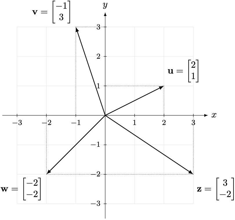
Throughout this post, let K denote any set and \mathbb K denote any field, which roughly speaking refers to any set where addition, subtraction, multiplication, and division is sufficiently well-defined.

Definition 1. The two-dimensional K-space is defined to be

K^2 \equiv K \times K := \left\{ \begin{bmatrix} x \\ y \end{bmatrix} : x \in K, y \in K\right\},

where we will denote the ordered pairs in column notation. In particular, \mathbb R^2 denotes the two-dimensional real space that we all know and love.

Very soon we will discuss ideas in much broader generality. But perhaps to motivate the subject, we can recall our usual vector operations that correspond to two-dimensional vectors used in high school physics.

Definition 2. Define addition and scalar multiplication on \mathbb K^2 via

\begin{bmatrix} u_1 \\ u_2 \end{bmatrix} + \begin{bmatrix} v_1 \\ v_2 \end{bmatrix} := \begin{bmatrix} u_1 + v_1 \\ u_2 + v_2 \end{bmatrix},\quad c\begin{bmatrix} v_1 \\ v_2 \end{bmatrix} := \begin{bmatrix} cv_1 \\ cv_2 \end{bmatrix}  ,\quad c \in \mathbb K.

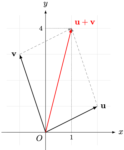
We expect these objects to behave like the vectors that we are familiar with, that in essence, encode directed distance. We call the set of these vectors a vector space.

Theorem 1. Let V = \mathbb K^2. Then V satisfies the following additive properties:

  • For \mathbf u, \mathbf v \in V, \mathbf u + \mathbf v \in V.
  • For \mathbf u, \mathbf v, \mathbf w \in V, \mathbf u + (\mathbf v + \mathbf w) = (\mathbf u + \mathbf v) + \mathbf w.
  • There exists an element \mathbf 0 \in V such that for any \mathbf v \in V, \mathbf v + \mathbf 0 = \mathbf v = \mathbf 0 + \mathbf v.
  • For any \mathbf v \in V, there exists an element -v \in V such that \mathbf v + (-\mathbf v) = (-\mathbf v) + \mathbf v = \mathbf 0.

In this case, we call V a group under +. In addition, we can add vectors in either order (i.e. this is the commutativity property):

  • For any \mathbf u, \mathbf v \in V, \mathbf u + \mathbf v = \mathbf v + \mathbf u.

In this case, we call V an abelian group under +. In addition, V satisfies the following scaling properties:

  • For any \mathbf v \in V and c, d \in \mathbb K, c(d\mathbf v) = (cd)\mathbf v.
  • For any \mathbf v \in V, 1\mathbf v = \mathbf v.
  • For \mathbf u, \mathbf v \in V and any c \in \mathbb K, c(\mathbf u + \mathbf v) = c\mathbf u + c\mathbf v.
  • For any \mathbf v \in V and c, d \in \mathbb K, (c+d)\mathbf v = c\mathbf v + d\mathbf v.

In this case, we call V a vector space over \mathbb K.

Proof Sketch. The proof is a matter of definition-checking. Nevertheless, we will complete some proofs to illustrate some of the techniques being used.

For the second property, we take advantage of the associativity of + in \mathbb K:

\begin{aligned} \begin{bmatrix} u_1 \\ u_2 \end{bmatrix}  + \left(\begin{bmatrix} v_1 \\ v_2 \end{bmatrix}  + \begin{bmatrix} w_1 \\ w_2 \end{bmatrix} \right) &= \begin{bmatrix} u_1 \\ u_2 \end{bmatrix}  + \begin{bmatrix} v_1 + w_1 \\ v_2 + w_2 \end{bmatrix} \\ &= \begin{bmatrix} u_1 + (v_1 + w_1) \\ u_2 + (v_2 + w_2) \end{bmatrix} \\ &= \begin{bmatrix} (u_1 + v_1) + w_1 \\ (u_2 + v_2) + w_2 \end{bmatrix} \\ &= \begin{bmatrix} u_1+v_1 \\ u_2+v_2 \end{bmatrix} + \begin{bmatrix} w_1 \\ w_2 \end{bmatrix} \\ &= \left( \begin{bmatrix} u_1 \\ u_2 \end{bmatrix}  + \begin{bmatrix} v_1 \\ v_2 \end{bmatrix} \right)  + \begin{bmatrix} w_1 \\ w_2 \end{bmatrix}. \end{aligned}

For the third property, we define \mathbf 0 := \begin{bmatrix} 0 \\ 0 \end{bmatrix} and check that it satisfies the required equations. For the fourth property, we define -\begin{bmatrix} v_1 \\ v_2 \end{bmatrix} := \begin{bmatrix} -v_1 \\ -v_2 \end{bmatrix} and do the needful bookkeeping.

Notice that this idea is not unique to \mathbb K^2. It could apply to many, many other sets, as we are about to see.

Lemma 1. For any field \mathbb L \supseteq \mathbb K, \mathbb L forms a vector space over \mathbb K. In particular, \mathbb K forms a vector space over \mathbb K.

Arguably the most important instances of vector spaces would be the function spaces. These spaces don’t always share all of the same properties as \mathbb R^2, but when they do, share these properties in a beautifully unified manner.

Theorem 2. For any vector space V over \mathbb K, let \mathcal F(K, V) denote the set of V-valued functions on K. Define addition and scalar multiplication according to the vector space structure of V:

For any f, g \in \mathcal F(K, V) and c \in \mathbb K,

(f +g)(x) := f(x) + g(x),\quad (cf)(x) := cf(x).

Then \mathcal F(K, V) forms a vector space over \mathbb K with additive identity 0 : K \to V defined by

0(x) = 0,\quad x \in K

and for any f \in \mathcal F(K, V), additive inverse -f : K \to V defined by

(-f)(x) = -f(x),\quad x \in K.

In particular, \mathcal F(\{1, 2\}, \mathbb K) forms a vector space over \mathbb K.

It is this last example that we want to emphasise as the twin brother of \mathbb K^2.

Theorem 3. For any \mathbf v = \begin{bmatrix} v_1 \\ v_2 \end{bmatrix} \in \mathbb K^2, define f_{\mathbf v} \in \mathcal F(\{1, 2\}, \mathbb K) by

f_{\mathbf v}(1) = v_1,\quad f_{\mathbf v}(2) = v_2.

Then the function T : \mathbb K^2 \to \mathcal F(\{1, 2\}, \mathbb K) defined by T( \mathbf v ) = f_{\mathbf v} satisfies the following property:

For any \mathbf u, \mathbf v \in \mathcal \mathbb K^2 and c \in \mathbb K,

T(\mathbf u + \mathbf v)= T(\mathbf u) + T(\mathbf v),\quad T(c\mathbf v) := cT(\mathbf v).

In this case, we call T a linear transformation. In addition, T is bijective, and we call T a vector space isomorphism. Therefore, we can write \mathbb K^2 = \mathcal F(\{1, 2\}, \mathbb K) without ambiguity.

Proof Sketch. The proof is immediate after we recognise that for each i = 1, 2,

f_{\mathbf u + \mathbf v}(i) = u_i + v_i = f_{\mathbf u}(i) +  f_{\mathbf v}(i) =  (f_{\mathbf u} + f_{\mathbf v})(i),

which implies that

T(\mathbf u+ \mathbf v) = f_{\mathbf u + \mathbf v} = f_{\mathbf u} + f_{\mathbf v} =T(\mathbf u) + T(\mathbf v).

The bijectivity of T is easily verifiable.

This connection allows us to define n-space as a function space.

Definition 3. For any vector space V over \mathbb K and n \geq 1, we define the vector space V^n := \mathcal F(\{1,\dots,n\}, V), which is a vector space over \mathbb K. In particular, \mathbb K^n = \mathcal F(\{1,\dots,n\}, \mathbb K), of which \mathbb R^n is a special case.

We insist on defining the vector space \mathcal F(K, V), since we can make remarkable connections with other areas of mathematics, as we will see in the next post.

—Joel Kindiak, 19 Feb 25, 2233H

,

Published by


Responses

  1. Differential Polynomials – KindiakMath

    […] that the linearity property of can be written […]

    Like

  2. Who Cares about Laplace Transforms? – KindiakMath

    […] them to commonly used solving techniques in future posts. Let’s first verify a familiar linearity property for the Laplace transforms that justifies the technique of […]

    Like

Leave a comment