The Magical Dot Product

Many linear algebra texts open with a definition of the dot product, say in three dimensions, as follows:

$\begin{bmatrix} u_1 \\ u_2 \\ u_3 \end{bmatrix} \cdot \begin{bmatrix} v_1 \\ v_2 \\ v_3 \end{bmatrix} := u_1 v_1 + u_2 v_2 + u_3 v_3.$

But where on earth did this formula arise from? Other authors open with a geometric definition with the dot product, but I shall open with a simple question: Given two vectors $\mathbf u, \mathbf v \in \mathbb R^2$ in the two-dimensional space, what is the angle $\theta$ between $\mathbf u$ and $\mathbf v$ ?

Motivated by the Pythagorean theorem, we can define the length of a two-dimensional vector as follows.

Definition 1. Given $\mathbf v = \begin{bmatrix} v_1 \\ v_2 \end{bmatrix}$ , the norm of $\mathbf v$ is defined by

$\|\mathbf v \| := \sqrt{v_1^2 + v_2^2}.$

Intuitively, this quantity captures the length of $\mathbf v$ .

Consider two vectors $\mathbf u = \begin{bmatrix} u_1 \\ u_2 \end{bmatrix},\mathbf v = \begin{bmatrix} v_1 \\ v_2 \end{bmatrix} \in \mathbb R^2$ with norm $1$ . In algebraic terms, we have

$u_1^2 + u_2^2 = v_1^2 + v_2^2 = 1.$

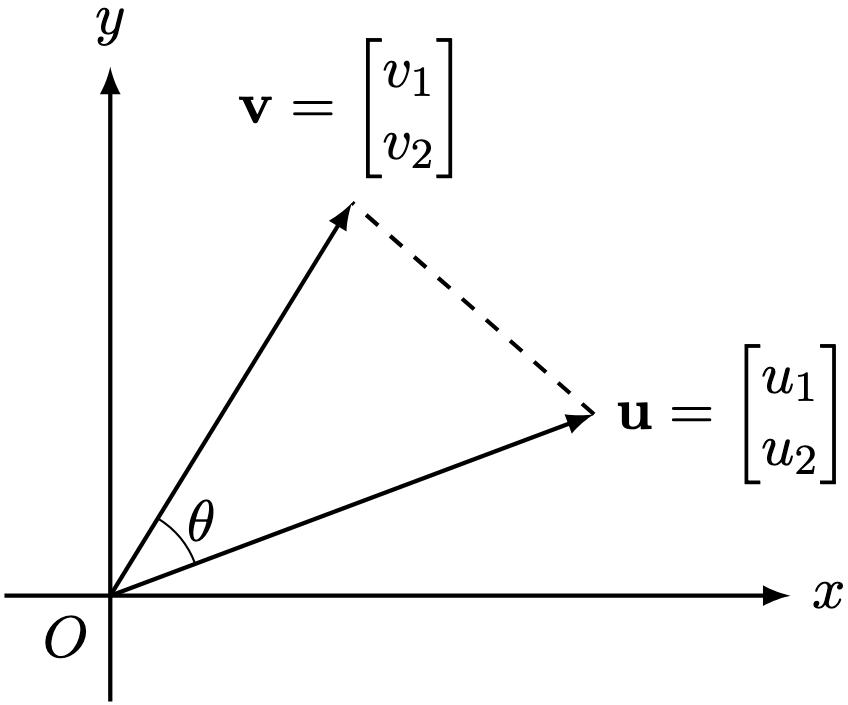
Assume $u_1 > v_1 > 0$ and $0 < u_2 < v_2$ for simplicity. Consider the triangle $\Delta OUV$ where $O(0, 0)$ , $U(u_1,u_2)$ , $V(v_1, v_2)$ . This means that

$\begin{aligned} \overrightarrow{VU} &= \overrightarrow{VO} + \overrightarrow{OU} = \overrightarrow{OU} - \overrightarrow{OV} \\ &= \begin{bmatrix} u_1 \\ u_2 \end{bmatrix} - \begin{bmatrix} v_1 \\ v_2 \end{bmatrix} = \begin{bmatrix} u_1 - v_1 \\ u_2 - v_2 \end{bmatrix}, \end{aligned}$

so that

$\begin{aligned} {VU}^2 &= (u_1 - v_1)^2 + (u_2 - v_2)^2 \\ &= (u_1^2 - 2 u_1 v_1 + v_1^2) + (u_2^2 - 2 u_2 v_2 + v_2^2) \\ &= (u_1^2 + u_2^2) + (v_1^2 + v_2^2) - 2(u_1 v_1 + u_2 v_2)\\ &= 1 + 1 - 2(u_1 v_1 + u_2 v_2) \\ &= 2 - 2(u_1 v_1 + u_2 v_2). \end{aligned}$

Letting $W$ be the foot of perpendicular from $V$ to $OU$ , we have $OW = \cos(\theta)$ and $WU = 1 - \cos(\theta)$ . By Pythagoras’ theorem,

${VW}^2 = {OV}^2 - {OW}^2 = {VU}^2 - {WU}^2.$

Substituting the relevant quantities,

$\begin{aligned} 1 - \cos^2(\theta) &= 2 - 2(u_1 v_1 + u_2 v_2) - (1-\cos(\theta))^2 \\ &= 2 - 2(u_1 v_1 + u_2 v_2) - (1 - 2 \cos(\theta) + \cos^2(\theta)) \\ &= 2 - 2(u_1 v_1 + u_2 v_2) - 1 + 2 \cos(\theta) - \cos^2(\theta) \\ &= 1 - \cos^2(\theta) + 2(\cos(\theta) - (u_1 v_1 + u_2 v_2)). \end{aligned}$

Since the $1 - \cos^2(\theta)$ terms cancel, we are left with the equality

$u_1 v_1 + u_2 v_2 = \cos(\theta).$

Therefore, the angle between $\mathbf u, \mathbf v$ can be computed using the sum-product $u_1 v_1 + u_2 v_2$ , which we abbreviate by the dot product notation

$\mathbf u \cdot \mathbf v := u_1 v_1 + u_2 v_2 = \cos(\theta).$

$\displaystyle \frac{ \mathbf u }{ \| \mathbf u \| } \cdot \frac{\mathbf v}{\| \mathbf v \|} = \cos(\theta),$

and if familiar algebraic calculations hold,

$\mathbf u \cdot \mathbf v = \| \mathbf u \| \| \mathbf v \| \cos(\theta).$

Yet, the dot product is itself of considerable interest. We can generalise it and talk about angles between other kinds of objects using this idea. This generalisation also features heavily in scientific applications like regression analysis. We can even use the dot product to give a theoretically useful meaning to the transpose of a matrix. More on these ideas in future posts.

Theorem 1. For any two vectors $\mathbf u = \begin{bmatrix} u_1 \\ u_2 \end{bmatrix},\mathbf v = \begin{bmatrix} v_1 \\ v_2 \end{bmatrix} \in \mathbb R^2$ in two-dimensional space, define their dot product by

$\mathbf u \cdot \mathbf v := u_1 v_1 + u_2 v_2$ .

The dot product satisfies the following properties:

For any $\mathbf v \in \mathbb R^2$ , $\mathbf v \cdot \mathbf v \geq 0$ .
For any $\mathbf v \in \mathbb R^2$ , $\mathbf v \cdot \mathbf v = 0$ implies $\mathbf v = \mathbf 0$ .
For any $\mathbf u, \mathbf v \in \mathbb R^2$ , $\mathbf u \cdot \mathbf v = \mathbf v \cdot \mathbf u$ .
For any $\mathbf u, \mathbf v \in \mathbb R^2$ , defining $\langle \cdot , \cdot \rangle : \mathbb R^2 \times \mathbb R^2 \to \mathbb R$ by $\langle \mathbf u, \mathbf v \rangle := \mathbf u \cdot \mathbf v$ , the functions $\langle \mathbf u, \cdot \rangle$ and $\langle \cdot, \mathbf v \rangle$ are linear over $\mathbb R$ .

Furthermore, if $u_1^2 + u_2^2 = v_1^2 + v_2^2 = 1$ , then $\mathbf u \cdot \mathbf v = \cos(\theta)$ . Consequently, for nonzero $\mathbf u,\mathbf v \in V$ ,

$\mathbf u \cdot \mathbf v = \| \mathbf u \| \| \mathbf v \| \cos(\theta).$

Proof. The second property is slightly tricky. Fix $\mathbf v \in \mathbb R^2$ . Then

$\mathbf v \cdot \mathbf v = 0 \quad \Rightarrow \quad 0 \leq v_1^2 = v_1^2 + v_2^2 = 0.$

Hence, $v_1 = 0$ . Similarly, $v_2 = 0$ . Therefore, $\mathbf v = \mathbf 0$ .

The dot product motivates the defining properties of the inner product, which we formulate to generalise the dot product.

Let $\mathbb K$ be either $\mathbb R$ or $\mathbb C$ .

Definition 1. A map $\langle \cdot , \cdot \rangle : V \times V \to \mathbb K$ is said to be an inner product on $V$ if it satisfies the following properties:

For any $\mathbf v \in V$ , $\langle \mathbf v, \mathbf v \rangle \in \mathbb R_{\geq 0}$ .
For any $\mathbf v \in V$ , $\langle \mathbf v, \mathbf v \rangle = 0$ implies $\mathbf v = \mathbf 0$ .
For any $\mathbf u, \mathbf v \in V$ , $\langle \mathbf u, \mathbf v \rangle = \overline{\langle \mathbf v, \mathbf u \rangle}$ . When $\mathbb K = \mathbb R$ , we recover usual symmetry.
For any $\mathbf v \in V$ , the map $\langle \cdot ,\mathbf v \rangle : V \to \mathbb K$ is linear.

The pair $V \equiv (V, \langle \cdot, \cdot \rangle)$ is called a $\mathbb K$ –inner product space.

Corollary 1. The dot product of two-dimensional vectors (i.e. in $\mathbb R^2$ ) as defined in Theorem 1 forms an inner product space.

Henceforth, suppose $\langle \cdot, \cdot \rangle$ is an inner product on $V$ .

Lemma 1. For any $\mathbf v \in V$ , define the quadrance of $\mathbf v$ by

$Q(\mathbf v) := \langle \mathbf v, \mathbf v \rangle \in \mathbb R_{\geq 0}.$

The following properties hold:

For any $\mathbf v \in V$ , $Q(\mathbf v) \in \mathbb R_{\geq 0}$ .
For any $\mathbf v \in V$ , $Q(\mathbf v) = 0$ implies $\mathbf v = \mathbf 0$ .
For any $\mathbf v \in V$ , $\alpha \in \mathbb K$ , $Q(\alpha \mathbf v) = |\alpha|^2 Q(\mathbf v)$ .

Proof. For the third property, we have

$\begin{aligned}Q(\alpha \mathbf v) &= \langle \alpha \mathbf v, \alpha \mathbf v \rangle = \alpha \langle \mathbf v, \alpha \mathbf v \rangle \\ &= \alpha \overline{ \langle \alpha \mathbf v, \mathbf v \rangle } = \alpha \overline{ \alpha \langle \mathbf v, \mathbf v \rangle } \\ &= \alpha \overline{\alpha} \overline{ \langle \mathbf v, \mathbf v \rangle } = |\alpha|^2 \langle \mathbf v, \mathbf v \rangle = |\alpha|^2 Q(\mathbf v). \end{aligned}$

Lemma 2 (Cauchy-Schwarz Inequality). For any $\mathbf u, \mathbf v \in V$ ,

$|\langle \mathbf u, \mathbf v \rangle |^2 \leq Q(\mathbf u) Q(\mathbf v).$

Proof. Fix $\mathbf u, \mathbf v \in V$ . If either $\mathbf u$ or $\mathbf v$ are $\mathbf 0$ , define $\alpha := 1$ . Otherwise, define

$\displaystyle \alpha := \frac{ | \langle \mathbf u,\mathbf v \rangle | }{\langle \mathbf u,\mathbf v \rangle}.$

In either instance, we have $|\alpha| = 1$ and $\alpha \langle \mathbf u,\mathbf v \rangle = | \langle \mathbf u,\mathbf v \rangle |$ .

Define the function $f_{\alpha} : \mathbb R \to \mathbb R_{\geq 0}$ by

$f_{\alpha}(t) := Q( \alpha t \mathbf u + \mathbf v).$

By expanding the definition of $Q$ , we obtain

$\begin{aligned} f_{\alpha}(t) &= \alpha \bar \alpha Q(\mathbf u) t^2 + (\alpha \langle \mathbf u, \mathbf v \rangle + \bar \alpha \langle \mathbf v, \mathbf u \rangle )t + Q(\mathbf v) \\ &= |\alpha|^2 Q(\mathbf u) t^2 + (| \langle \mathbf u,\mathbf v \rangle | + | \langle \mathbf u,\mathbf v \rangle | )t + Q(\mathbf v) \\ &= Q(\mathbf u) t^2 +2 | \langle \mathbf u,\mathbf v \rangle | t + Q(\mathbf v).\end{aligned}$

Since $f_{\alpha}(t) \geq 0$ for any $t \in \mathbb R$ , we must have

$( 2 | \langle \mathbf u,\mathbf v \rangle | )^2 - 4 Q(\mathbf u) Q(\mathbf v) \leq 0,$

yielding $|\langle \mathbf u, \mathbf v \rangle |^2 \leq Q(\mathbf u) Q(\mathbf v)$ .

Theorem 2. For any $\mathbf v \in V$ , define the norm of $\mathbf v$ by $\| \mathbf v\| := \sqrt{ Q( \mathbf v ) }$ . The following properties hold:

For any $\mathbf v \in V$ , $\| \mathbf v \| \geq 0$ .
For any $\mathbf v \in V$ , $\| \mathbf v \| = 0$ implies $\mathbf v = \mathbf 0$ .
For any $\mathbf v \in V$ , $\alpha \in \mathbb K$ , $\|\alpha \mathbf v \| = |\alpha| \| \mathbf v \|$ .
For any $\mathbf u, \mathbf v \in V$ , $\|\mathbf u + \mathbf v \| \leq \| \mathbf u \| + \| \mathbf v \|$ .

We call $V \equiv (V, \| \cdot \| )$ a normed space.

Proof. For the last result, we use the Cauchy-Schwarz inequality to derive that

$\begin{aligned} \|\mathbf u + \mathbf v \|^2 &= Q(\mathbf u + \mathbf v) \\ &= Q( \mathbf u )+ \langle \mathbf u,\mathbf v \rangle + \langle \mathbf v,\mathbf u \rangle + Q( \mathbf v ) \\ &= \| \mathbf u \|^2 + 2\, \text{Re}(\langle \mathbf u,\mathbf v \rangle) + \| \mathbf v \|^2 \\ &\leq \| \mathbf u \|^2 + 2 \| \mathbf u \| \| \mathbf v \| + \| \mathbf v \|^2 \\ &= (\| \mathbf u \| + \| \mathbf v \| )^2, \end{aligned}$

where we defined $\mathrm{Re}(x+iy) := x$ for $x,y \in \mathbb R$ , and observe that for any $z \in \mathbb C$ , $-|z| \leq \mathrm{Re}(z) \leq |z|$ .

Corollary 2. For any nonzero $\mathbf v \in V$ , define the unit vector $\hat{\mathbf v}$ of $\mathbf v$ by

$\displaystyle \hat{\mathbf v} := \frac{ \mathbf v }{ \| \mathbf v \| }.$

Then $\|\hat{\mathbf v}\| = 1$ . In particular, if $\mathbb K = \mathbb R$ , for nonzero $\mathbf u, \mathbf v$ , define the angle between them $\theta \in [0, \pi]$ by

$\theta := \cos^{-1} (\langle \hat{\mathbf u}, \hat{\mathbf v} \rangle).$

Then $\langle \mathbf u, \mathbf v \rangle = \| \mathbf u \| \| \mathbf v \| \cos(\theta)$ .

Proof. For the final result, we note that $\mathbf u = \| \mathbf u \| \hat{\mathbf u}$ . Then

$\langle \mathbf u, \mathbf v \rangle = \langle \| \mathbf u \| \hat{\mathbf u} , \| \mathbf v \| \hat{\mathbf v} \rangle = \| \mathbf u \| \| \mathbf v \| \langle \hat{\mathbf u}, \hat{\mathbf v} \rangle = \| \mathbf u \| \| \mathbf v \| \cos(\theta).$

Corollary 3. Define the metric $d : V \times V \to \mathbb R$ by the map

$d(\mathbf u,\mathbf v) := \|\mathbf u - \mathbf v \|.$

The following properties hold:

For any $\mathbf u,\mathbf v \in V$ , $d(\mathbf u, \mathbf v) \geq 0$ .
For any $\mathbf v \in V$ , $d(\mathbf v, \mathbf v) = 0$ implies $\mathbf v = \mathbf 0$ .
For any $\mathbf u,\mathbf v \in V$ , $d(\mathbf u, \mathbf v) = d(\mathbf v, \mathbf u)$ .
For any $\mathbf u, \mathbf v, \mathbf w \in V$ , $d(\mathbf u,\mathbf v) \leq d(\mathbf u, \mathbf w) + d(\mathbf w, \mathbf v)$ .

We call $V \equiv (V, d )$ a metric space.

Proof. For the last result, use the observation

$\mathbf u - \mathbf v = (\mathbf u - \mathbf w) + (\mathbf w - \mathbf v).$

Therefore, all inner product spaces are normed spaces, and all normed spaces are metric spaces. By some further investigation, every metric space forms a topological space too. If we took a different generalisation from the usual narrative, we would have explored the notion that all normed spaces are topological vector spaces, which in turn are topological spaces.

Each generalisation has their uses in modern mathematics, but for now, let’s focus on inner product spaces. We will first explore the theory of inner product spaces before exploring their ubiquitous applications across mathematics.

—Joel Kindiak, 12 Mar 25, 1407H

KindiakMath

The Magical Dot Product

Leave a comment Cancel reply

The Magical Dot Product

Share this:

Leave a comment Cancel reply