Let’s try to make some money.
You want to earn money by selling fidget spinners, but two questions arise:
- How much revenue can you earn by selling the fidget spinners?
- How much cost would you incur by obtaining the fidget spinners in the first place?
Your profit is then defined by

Let’s first investigate your potential costs.
Example 1. Suppose you buy fidget spinners at a unit cost of 
represents the number of fidget spinners you obtain.
represents the total cost of buying
What would be the relationship between 
Solution. Using basic counting,

Hence, 


Example 2. In Example 1, if you can spend a maximum of 
Solution. Since the maximum cost is capped at 

We need to determine the number that 


Therefore, 
Remark 1. Suppose you had 

produces the value 
- We may be tempted to reject the answer
of a fidget spinner doesn’t arise in real life.
- However, if
, then the answer
fidget spinners—a perfectly reasonable solution!
Therefore, in general, we can accept non-whole number values of
Example 3. If you need to pay a fixed delivery fee of 
Solution. By including the delivery fee,

For example, if 


using the usual order of operations.
We can picture this relationship using a graph.
- The horizontal right arrow, called the
- The vertical up arrow, called the
If we allowed 

We recover a straight line!
Example 4. Calculate the change in cost incurred by obtaining one additional fidget spinner. This change is called the gradient of the graph.
Solution. Let 

By incrementing the number of fidget spinners, we want to buy 


Hence, the required change in cost is

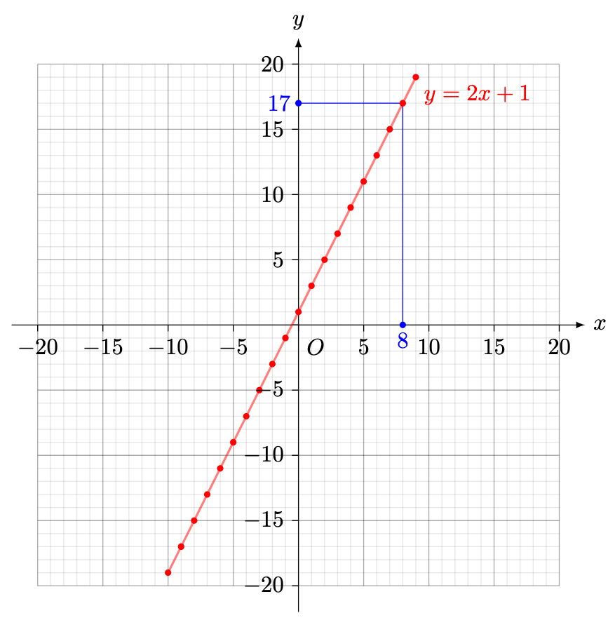
Example 5. Using 
Solution. Setting 

Definition 1. A graph is called a (non-vertical) straight line with:
- gradient
,
,
if it is continuously drawn using the equation

The value
- if
, then the line is upward-sloping,
- if
, then the line is horizontal,
- if
, then the line is downward-sloping.
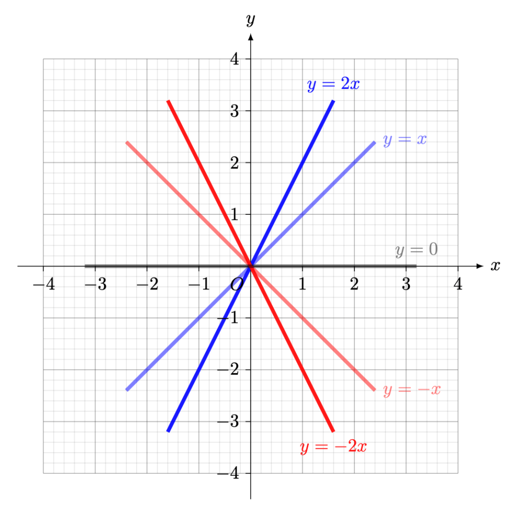
Furthermore,
- the more positive the gradient, the steeper the increase,
- the more negative the gradient, the steeper the decrease.
The value
- if
- if
- if
If
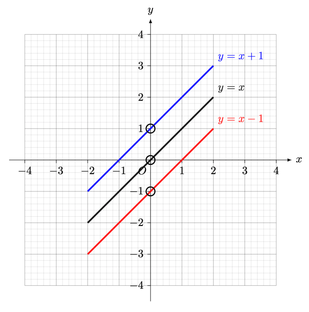
In short,
Definition 2. Define a point as a position in space described by a pair of real numbers, denoted 
Lemma 1. If two points 


Proof Sketch. Let the non-vertical straight line have equation 

We leave it as an exercise to check that

Lemma 2. The equation of a non-vertical straight line passing through the point

Proof Sketch. Using Lemma 1, any point 

Hence, 
Example 6. You discover that:
per fidget spinner,
people are willing to pay
per fidget spinner.
Let
Stating your assumptions, determine a reasonable relationship between
Solution. We can picture the two situations in the graph below.
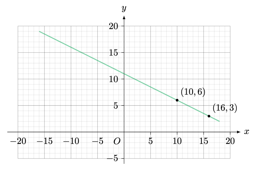
By assuming a straight-line (i.e. linear) graph, we will first apply Lemma 1 using the points 


Since the straight line passes through

Hence, 
Definition 3. A graph is a vertical line with 

Example 7. The line 
Definition 4. A graph is called a straight line if it can be continuously drawn using the linear equation 

Theorem 1. A graph is a straight line if and only if it is either a vertical line or a non-vertical straight line.
Proof Sketch. We notice either 

- Using Definition 3,
- Using Definition 1,
The complete proof using the definitions is left as a good exercise in algebraic manipulation.
Remark 2. This blog post is inspired by ideas in business and economics:
- Example 3 pictures the supply curve: how much you are willing to pay in order to sell
- Example 6 pictures the demand curve: how much people are willing to pay in order to buy
Let’s now draw Example 3 and Example 6 on the same graph.

What is the maximum number of fidget spinners that would be worth selling?
Obviously, when the two graphs intersect!
By using our eyeballs (i.e. inspection), the point of intersection has coordinates 
—Joel Kindiak, 27 Sept 25, 1450H

Leave a reply to Baby Linear Algebra – KindiakMath Cancel reply