The Curvy Gradient

Calculus, in the 21st century, continues to be the sorrow of most students required to learn it against their will. It doesn’t need to be this way, though.

Consider the graph of $y = x^2$ below.

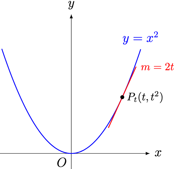
Define the point $P_t$ on the graph by $(t, t^2)$ . Using algebra, we can evaluate the gradient of the tangent at $P_t$ to $2t$ .

Now consider the graph of $y =x^3$ .

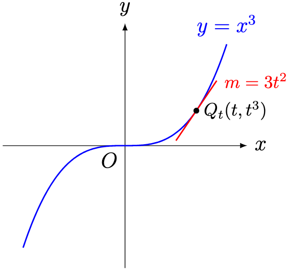
Define the point $Q_t$ on the graph by $(t, t^3)$ . Using algebra, we can evaluate the gradient of the tangent at $Q_t$ to $3t^2$ .

We are going to generalise this observation.

Definition 1. Let $y = f(x)$ be the graph of a function. The derivative of $f(x)$ at $x = t$ , denoted $f'(t)$ , is defined to be the gradient of the tangent at $(t, f(t))$ .

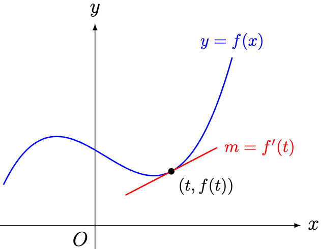
Define the derivative of $f(x)$ by

$\displaystyle \frac{\mathrm d}{\mathrm dx}(f(x)) := f'(x).$

Since $y = f(x)$ , we can also write

$\displaystyle \frac{\mathrm dy}{\mathrm dx} \equiv \frac{\mathrm d}{\mathrm dx}(y) \equiv \frac{\mathrm d}{\mathrm dx}(f(x)).$

We describe this process as differentiating $f(x)$ with respect to $x$ .

Remark 1. Strictly speaking, the derivative is defined as a limit, and the gradient of the tangent is defined to be the derivative. However, we adopt the convention in Definition 1 for the sake of visual intuition.

Using more mathematical tools to establish a common pattern, we will define the derivative of $x^n$ , where $n$ is any rational number.

Theorem 1. The derivative of $x^n$ with respect to $x$ is given by

$\displaystyle \frac{\mathrm d}{\mathrm dx}(x^n) := nx^{n-1}.$

Proof. See this post for the more formal perspective, and see this exercise for the algebraic calculation. We see that

$\displaystyle \frac{\mathrm d}{\mathrm dx}(x^2) = 2x,\quad \frac{\mathrm d}{\mathrm dx}(x^3) = 3x^2,$

and these results agree with our investigation in earlier examples.

Example 3. Evaluate the following derivatives:

$\displaystyle \frac{\mathrm d}{\mathrm dx}(x^4), \quad \frac{\mathrm d}{\mathrm dx}(x),\quad \frac{\mathrm d}{\mathrm dx}(1), \quad \frac{\mathrm d}{\mathrm dx} \left( \frac 1x \right),\quad \frac{\mathrm d}{\mathrm dx}(\sqrt x).$

Solution. The first expression is immediate using Theorem 1:

$\begin{aligned} \frac{ \mathrm d}{\mathrm dx}(x^4) &= 4x^{4-1} \\ &= 4x^3. \end{aligned}$

The second expression requires the two laws of exponents $x = x^1$ and $x^0 = 1$ :

$\begin{aligned} \frac{ \mathrm d}{\mathrm dx}(x) &= \frac{ \mathrm d}{\mathrm dx}(x^1) \\ &= 1x^{1-1} \\ &= 1x^0 \\ &= 1 \cdot 1 = 1. \end{aligned}$

The third expression requires $1 = x^0$ :

$\displaystyle \begin{aligned} \frac{ \mathrm d}{\mathrm dx}(1) &= \frac{ \mathrm d}{\mathrm dx}(x^0) \\ &= 0x^{0-1} \\ &= 0x^{-1} = 0. \end{aligned}$

The fourth expression requires $1/x = x^{-1}$ and more generally, $x^{-n} = 1/x^n$ :

$\begin{aligned} \frac{ \mathrm d}{\mathrm dx}\left( \frac 1x \right) &= \frac{ \mathrm d}{\mathrm dx}(x^{-1}) \\ &= (-1)x^{-1-1} \\ &= -x^{-2} = -\frac 1{x^2}. \end{aligned}$

The fifth expression requires $\sqrt x = x^{1/2}$ and $x^{-n} = 1/x^n$ :

$\begin{aligned} \frac{ \mathrm d}{\mathrm dx} (\sqrt x) &= \frac{ \mathrm d}{\mathrm dx}(x^{\frac 12}) \\ &= {\textstyle \frac 12} \cdot x^{\frac 12-1} \\ &= {\textstyle \frac 12} \cdot x^{-\frac 12} \\ &=\frac 1{2} \cdot \frac 1{x^{\frac 12}} \\ &= \frac 12 \cdot \frac 1{\sqrt x} = \frac 1{2\sqrt x}. \end{aligned}$

Is it possible to evaluate derivatives of combinations of these functions? Yes!

Theorem 2. Given functions $f(x), g(x)$ and constants $a, b$ ,

$\displaystyle \frac{\mathrm d}{\mathrm dx}(a \cdot f(x) + b \cdot g(x)) = a \cdot \frac{\mathrm d}{\mathrm dx}(f(x)) + b \cdot \frac{\mathrm d}{\mathrm dx}(g(x)).$

Proof. See this post from a calculus perspective and this post from a linear-algebra perspective. This result is known as the linearity of the derivative.

Example 4. Given functions $f(x), g(x), h(x)$ , show that

$\displaystyle \frac{\mathrm d}{\mathrm dx}( f(x) + g(x) + h(x) ) = \frac{\mathrm d}{\mathrm dx}(f(x)) + \frac{\mathrm d}{\mathrm dx}(g(x)) + \frac{\mathrm d}{\mathrm dx}(h(x)).$

Solution. Using the linearity of the derivative,

$\begin{aligned} &\frac{\mathrm d}{\mathrm dx}( f(x) + g(x) + h(x) ) \\ &= \frac{\mathrm d}{\mathrm dx}( (f(x) + g(x)) + h(x) ) \\ &= \frac{\mathrm d}{\mathrm dx}(f(x) + g(x)) + \frac{\mathrm d}{\mathrm dx}(h(x)) \\ &= \left(\frac{\mathrm d}{\mathrm dx}(f(x)) + \frac{\mathrm d}{\mathrm dx}(g(x))\right) + \frac{\mathrm d}{\mathrm dx}(h(x)) \\ &= \frac{\mathrm d}{\mathrm dx}(f(x)) + \frac{\mathrm d}{\mathrm dx}(g(x)) + \frac{\mathrm d}{\mathrm dx}(h(x)).\end{aligned}$

Example 5. Evaluate the following derivatives:

$\displaystyle \frac{\mathrm d}{\mathrm dx}( x^2 + 2x + 1 ),\quad \frac{\mathrm d}{\mathrm dx}( (x+1)^2 ),\quad \frac{\mathrm d}{\mathrm dx}( (x+1)^3 ).$

Solution. For the first expression, we use linearity as per Example 4:

$\begin{aligned} \frac{\mathrm d}{\mathrm dx}( x^2 + 2x + 1 ) &= \frac{\mathrm d}{\mathrm dx}(x^2) + 2 \cdot \frac{\mathrm d}{\mathrm dx}(x) + \frac{\mathrm d}{\mathrm dx}(1). \end{aligned}$

Using the results in Theorem 1 and Example 3, we have

$\begin{aligned} \frac{\mathrm d}{\mathrm dx}( x^2 + 2x + 1 ) &= \frac{\mathrm d}{\mathrm dx}(x^2) + 2 \cdot \frac{\mathrm d}{\mathrm dx}(x) + \frac{\mathrm d}{\mathrm dx}(1) \\ &= 2x + 2 \cdot 1 + 0 \\ &= 2x + 2. \end{aligned}$

For the second expression, we expand $(x+1)^2$ , then use the previous answer:

$\begin{aligned} \frac{\mathrm d}{\mathrm dx}( (x+1)^2 ) = \frac{\mathrm d}{\mathrm dx}( x^2 + 2x + 1 ) = 2x + 2 \end{aligned}$

For the third expression, we first expand $(x+1)^3$ :

$\begin{aligned} (x+1)^3 &= (x+1)^2 \cdot (x+1) \\ &= (x^2 + 2x + 1)(x + 1) \\ &= x^3 + (2 + 1)x^2 + (1+2)x + 1 \\ &= x^3 + 3x^2 + 3x + 1.\end{aligned}$

We then use linearity and established results as per Theorem 1 and Example 3:

$\begin{aligned} \frac{\mathrm d}{\mathrm dx}( (x+1)^3 ) &= \frac{\mathrm d}{\mathrm dx}( x^3 + 3x^2 + 3x + 1 ) \\ &= \frac{\mathrm d}{\mathrm dx}(x^3) + 3 \cdot \frac{\mathrm d}{\mathrm dx}(x^2) + 3 \cdot \frac{\mathrm d}{\mathrm dx}(x) + \frac{\mathrm d}{\mathrm dx}(1) \\ &= 3x^2 + 3 \cdot 2x + 3 \cdot 1 + 0 \\ &= 3x^2 + 6x + 3. \end{aligned}$

To shorten notation, we write $f'(x) = \displaystyle \frac{\mathrm d}{\mathrm dx}(f(x))$ .

Example 6. Given functions $f(x), g(x)$ , show that

$\displaystyle \frac{\mathrm d}{\mathrm dx}( f(x) - g(x) ) = \displaystyle f'(x) - g'(x).$

Solution. Since $f(x) - g(x) = f(x) + (-1) \cdot g(x)$ , we use linearity to derive

$\begin{aligned} \frac{\mathrm d}{\mathrm dx}( f(x) - g(x) ) &= \frac{\mathrm d}{\mathrm dx}( f(x) + (- 1) \cdot g(x) ) \\ &= \frac{\mathrm d}{\mathrm dx}( f(x) ) + (- 1) \cdot \frac{\mathrm d}{\mathrm dx} ( g(x) ) \\ &= f'(x) + (-1) \cdot g'(x) \\ &= f'(x) - g'(x).\end{aligned}$

Example 7. Let $a, b$ be positive constants. In economics, the revenue $R$ earned from selling $x$ units of a good is given by

$R \equiv R(x) = x(a - bx).$

Define the two quantities related to the revenue:

The average revenue is defined by $\mathrm{AR}(x) := R(x)/x$ .
The marginal revenue is defined by $\mathrm{MR}(x) := R'(x)$ .

Show that the $x$ -intercept of $y = \mathrm{MR}(x)$ is half of the $x$ -intercept of $y = \mathrm{AR}(x)$ .

Solution. By algebra, $\mathrm{AR}(x) = a-bx$ and

$\mathrm{R}(x) = x(a-bx) = ax - bx^2.$

Using linearity,

$\begin{aligned} \mathrm{MR}(x) &= \frac{\mathrm d}{\mathrm dx}(R(x)) \\ &= \frac{\mathrm d}{\mathrm dx}(ax - bx^2) \\ &= a \cdot \frac{\mathrm d}{\mathrm dx}(x) - b \cdot \frac{\mathrm d}{\mathrm dx}(x^2) \\ &= a \cdot 1 - b \cdot 2x \\ &= a - 2bx. \end{aligned}$

Let $x_1$ denote the $x$ -intercept of $y = \mathrm{AR}(x)$ and $x_2$ denote the $x$ -intercept of $y = \mathrm{MR}(x)$ .

We first solve $\mathrm{AR}(x_1) = 0$ :

$\begin{aligned} \mathrm{AR}(x_1) &= 0 \\ a - bx_1 &= 0 \\ x_1 &= \frac ab. \end{aligned}$

We next solve $\mathrm{MR}(x_2) = 0$ :

$\begin{aligned} \mathrm{MR}(x_2) &= 0 \\ a - 2bx_2 &= 0 \\ x_2 &= \frac a{2b}. \end{aligned}$

Hence, $2x_2 = 1/b = x_1$ , so that $x_2 = x_1/2$ .

What other combinations can we differentiate? Given functions $f(x), g(x)$ , we can differentiate the following:

$\displaystyle f(x) \cdot g(x),\quad \frac{ f(x) }{ g(x) },\quad f(g(x)).$

Tragically, they don’t follow the neat rules that we think they do.

Example 8. Which of the following equations are true?

$\begin{aligned} \frac{\mathrm d}{\mathrm dx}( f(x) \cdot g(x) ) &= f'(x) \cdot g'(x), \\ \frac{\mathrm d}{\mathrm dx} \left( \frac{ f(x) }{ g(x) } \right) &= \frac{ f'(x) }{ g'(x) }, \\ \frac{\mathrm d}{\mathrm dx} \left( f(g(x)) \right) &= f'(g(x)). \end{aligned}$

Justify your answer.

Solution. Sadly, none of them are true.

We will use the counter-example $f(x) = x^3$ and $g(x) = x^2$ . Using Theorem 1, $f'(x) = 3x^2$ and $g'(x) = 2x$ .

For the first equation,

$\displaystyle \frac{\mathrm d}{\mathrm dx}( f(x) \cdot g(x) ) = \frac{\mathrm d}{\mathrm dx}(x^3 \cdot x^2) = \frac{\mathrm d}{\mathrm dx}(x^5) = 5x^4,$

however,

$\displaystyle f'(x) \cdot g'(x) = 3x^2 \cdot 2x = 6x^3.$

Therefore,

$\displaystyle \frac{\mathrm d}{\mathrm dx}( f(x) \cdot g(x) ) = 6x^3 \neq 5x^4 = f'(x) \cdot g'(x).$

For the second result, we leave it as an exercise to check that

$\displaystyle \frac{\mathrm d}{\mathrm dx} \left( \frac{ f(x) }{ g(x) } \right) = 1 \neq \frac{3x}{2} = \frac{ f'(x) }{ g'(x) }.$

For the third result, we leave it as an exercise to check that

$\displaystyle \frac{\mathrm d}{\mathrm dx} ( f( g(x) ) ) = 6x^5 \neq 3x^4 = f'(g(x)).$

To deal with these latter three results, we will need to look at the three musketeers of differentiation techniques: the chain rule, the product rule, and the quotient rule. For more complete proofs, see this post on the chain rule and this post for the product and quotient rules.

We will explore this differentiation trio next time.

—Joel Kindiak, 7 Jan 26, 1450H

KindiakMath

The Curvy Gradient

Leave a comment Cancel reply

The Curvy Gradient

Share this:

Leave a comment Cancel reply