In this set of posts, we strategise over the mechanics behind a game of Blackjack.
Definition 1. A poker card deck comprises of 52 cards. Each card is uniquely characterised by two pieces of information: the value and the suit.
- The value is an element from the set {A, 2, 3, …, 10, J, Q, K}.
- The suit is chosen from the set {Clubs, Diamonds, Hearts, Spades}.
For each value, there exists 4 cards, one for each suit. Conversely, for each suit, there exists 13 cards, one for each value. Cards whose value belong to {J, Q, K} are called picture cards. The symbols J, Q, K denote Jack, Queen, and King respectively.
At the start of each round, two cards are dealt to the player without replacement.
Problem 1. Calculate the probability that the player’s hand contains two cards with the same value. We call this a double.
(Click for Solution)
Solution. Given each value A, 2, 3, …, 10, J, Q, K, the probability of a double is given by

Since there are 13 total values, the required probability is

In Blackjack, the goal is to achieve the highest total score subject to a maximum total of 21. More precisely, for each card with value  , define its score
  as follows:

Given the initial hand  with values
  , define its total score by

Problem 2. Evaluate the total score of the hand (K, 6).
(Click for Solution)
Solution. By definition,  .
.
For hands involving A (called Ace), define s(A) := 1. Furthermore,

Regard score-summing as commutative, so that s(v, A) = s(A, v).
Problem 3. Evaluate the total score of the hands (A, A), (A, 2), (A, K) respectively.
(Click for Solution)
Solution. In all hands,  . Therefore,

Definition 2. A player obtains a Blackjack if  .
.
Problem 4. Calculate the probability that a player obtains a Blackjack.
(Click for Solution)
Solution. We observe that a player with a hand  has a Blackjack if and only if at least one of the cards is an Ace, and the other has score 10. Therefore,

If a player does not get a Blackjack, he gets to choose to add one more card or stand. Given a hand  , define its total score by

If a player’s total score exceeds 21, we say that the player busts and loses immediately.
Problem 5. A player has an initial hand (K, 6). If the player chooses to hit and obtain a card w, what is the probability that he busts with the hand (K, 6, w)?
(Click for Solution)
Solution. Since there are no Aces, the player’s current score is 16 by Problem 2. Furthermore, s(A) = 1 with no extra additions by 10. Therefore,

If any hand has an Ace, define

A non-Blackjack hand that has an Ace and  is called a soft total.
Problem 6. Given an initial soft total (A, v), the player hits and obtains a card with value W. Calculate the probability that s(A, v, W) = 21.
(Click for Solution)
Solution. Since the total is soft, it is not a Blackjack, so that  . Regarding the second ace A as 1, for each
  ,
,  .
.

If  , then
  . Hence,

If  , then
  . Hence,

Each game is played against the dealer. The dealer will have one card exposed and the other card concealed. After the player no longer hits, the dealer will keep hitting until its score total exceeds 16, after which, the dealer is no longer allowed to add any more card.
Let  denote the probability that the dealer busts given that his initial hand
  has no Aces and an initial total
  .
.
Problem 7. Evaluate  .
.
(Click for Solution)
Solution. By definition, the dealer must bust in his next hit  , so
, so

Remark 1. These problems don’t even account for the reward system in Blackjack, which requires a more detailed analysis of expected values, or before that, the case when the dealer has a soft hand (e.g. Aces in his initial hand).
—Joel Kindiak, 5 Apr 26, 1847H


 , we defined its second derivative by the first derivative of the first derivative:

 , evaluate

 and
and  below.
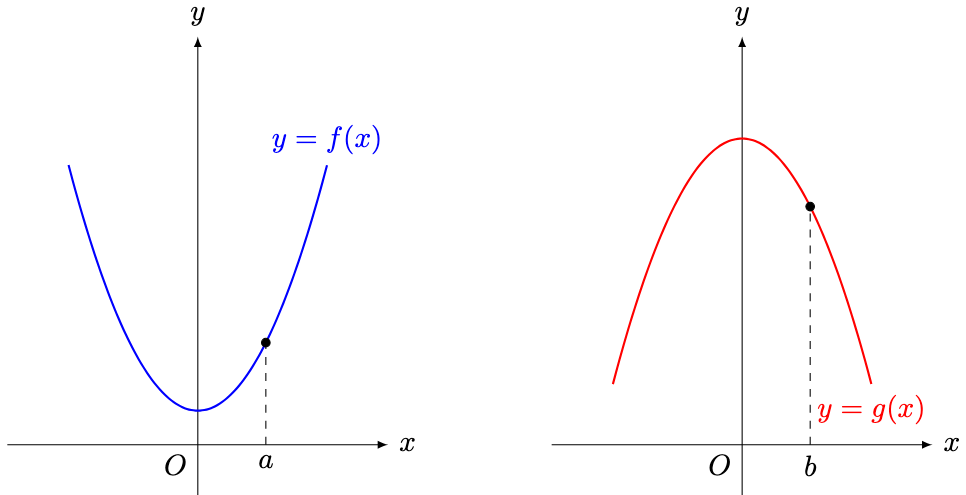
 and
and  . In this case, we say that
  is convex near
  and
and  is concave near
  .
. denote the tangent to
  with gradient
  . For some small
  ,
,  is steeper than
  , so that
  . Since
  is increasing from
  to
to  ,
,  denote the tangent to
  with gradient
  . For some small
  is steeper than
  , so that
  . Since
  is decreasing from
  to
to  ,
,  , evaluate
  .
.
 and
and  for
for  . What do you notice?
 ,
,
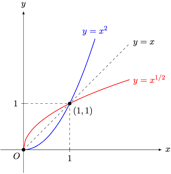
 and
and  , and are reflections of each other about the line
  .
. and
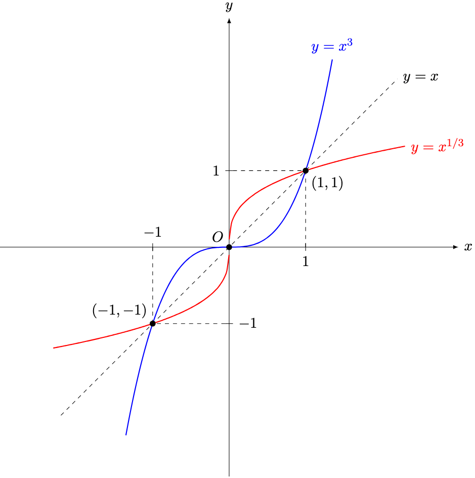
and  for
for  . What do you notice?

 ,
,
 ,
,  , show that if
  , then
  . Furthermore, if
  , then show that
 ,
,


 the subject,
 if
if  (i.e.
(i.e.  is convex near
  for
for 


 for
for 


 for any
  and
and  for
for  for any
 for
for  is always concave and increasing. Finally, as
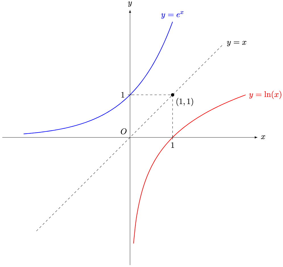
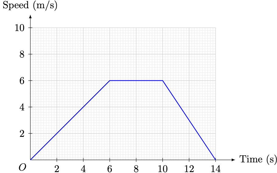
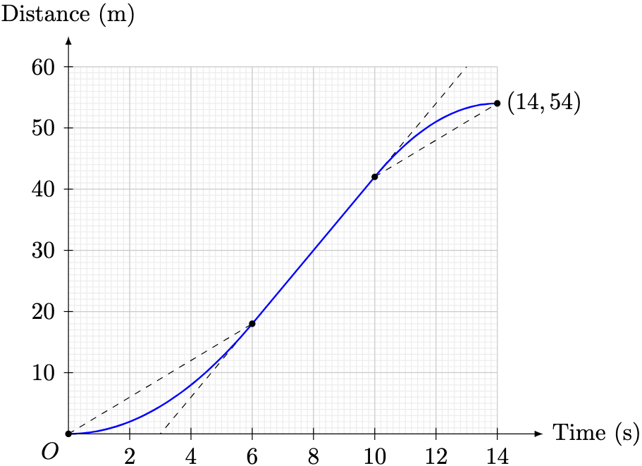
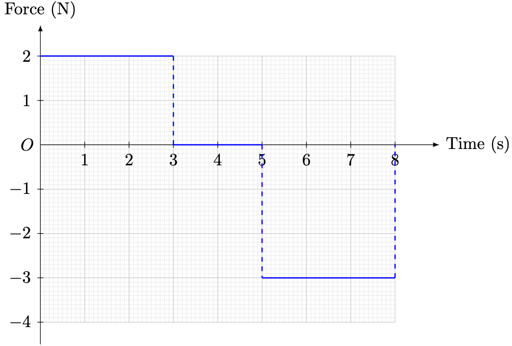
 denote the total distance travelled by the particle at time
  . Using the area under the graph,
 denote the acceleration of the particle at time
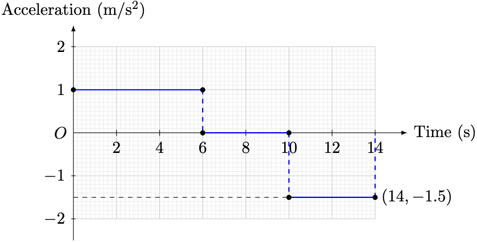
 is given by
 denote the total momentum of the object at time
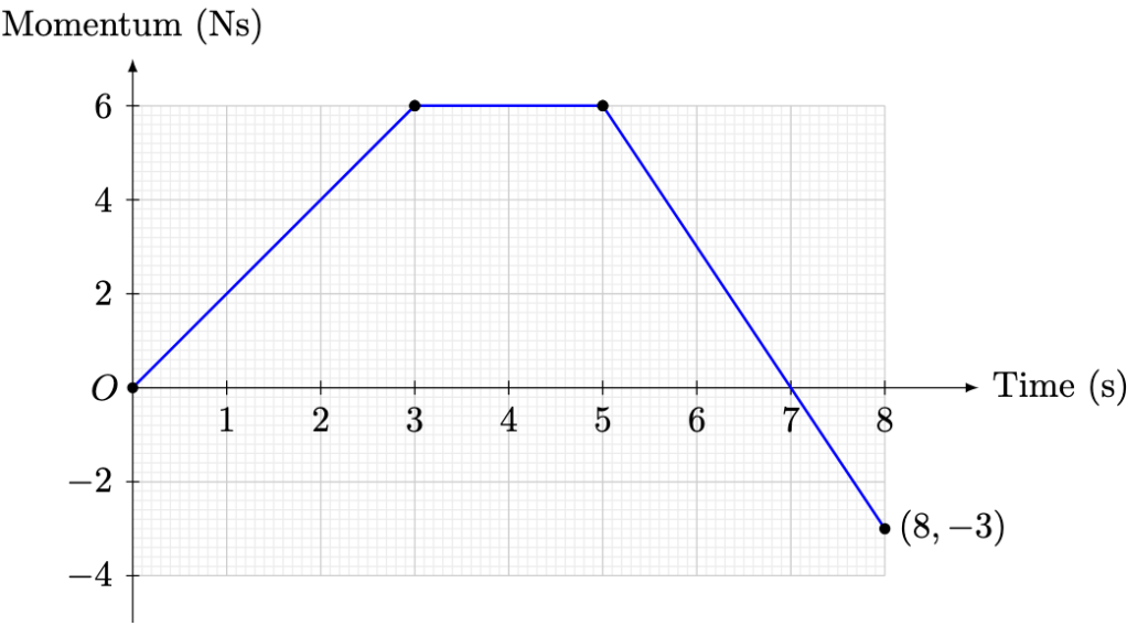
 . By the

 at
at  as follows.
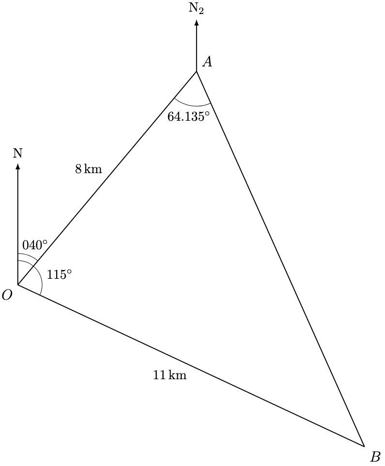
 ,
,
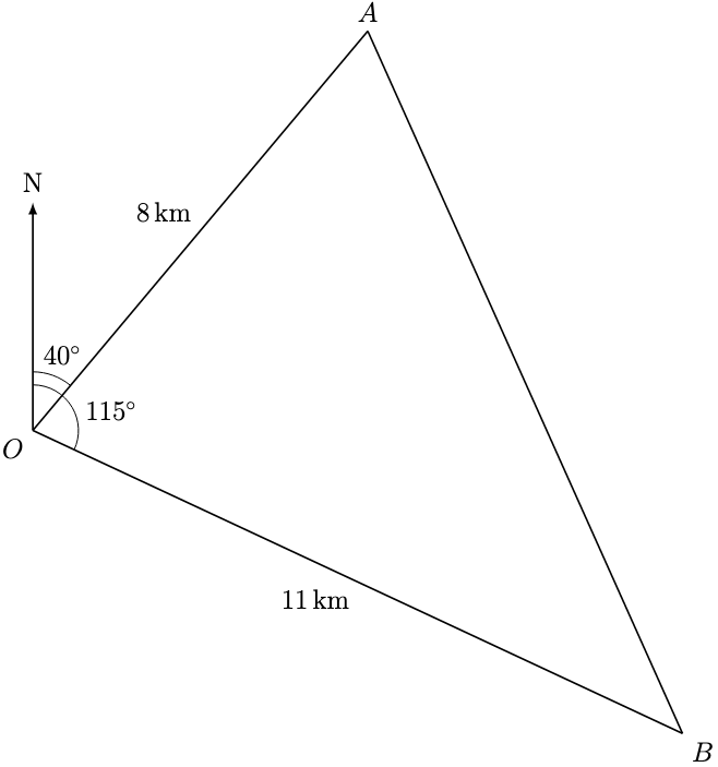
 , the required bearing is given by
 as follows. Similar, the angle of depression of G from T is defined by
  as follows.
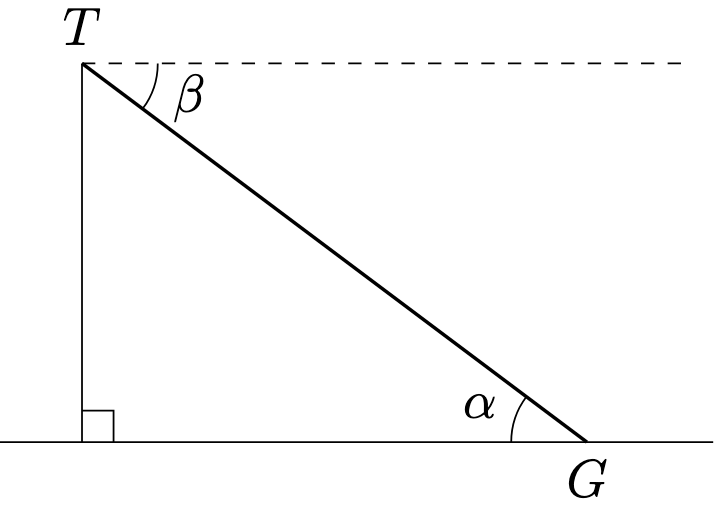
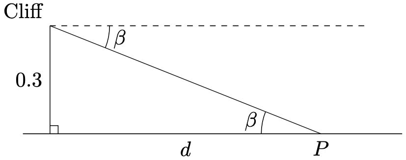
 denote the horizontal distance, in kilometres, from the coastguard station to
  .
.

 :
:


 .
. as follows.
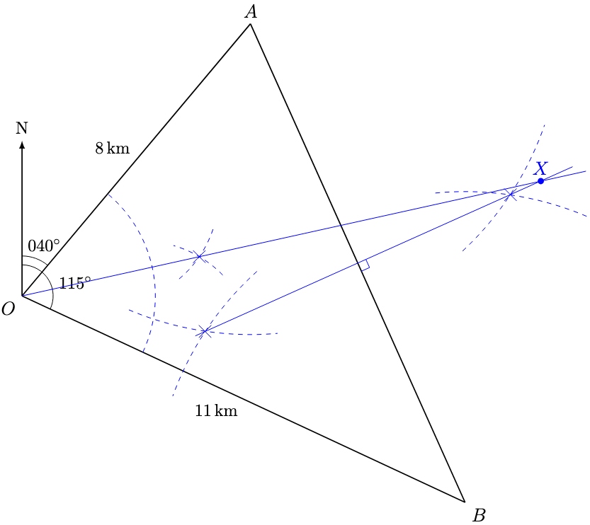
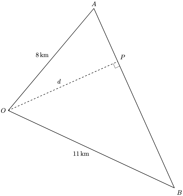
 denote the buoy, the required distance is approximately 12.0 km.
 and the standard deviation
  by
by


 .
.


 . Substituting all displays,
 ,
,
 ,
,


 ,
,  . Since
  and
and  , substituting the values yields
 .
.


 .
.
 , substituting into the display yields
  . Therefore,
  .
.
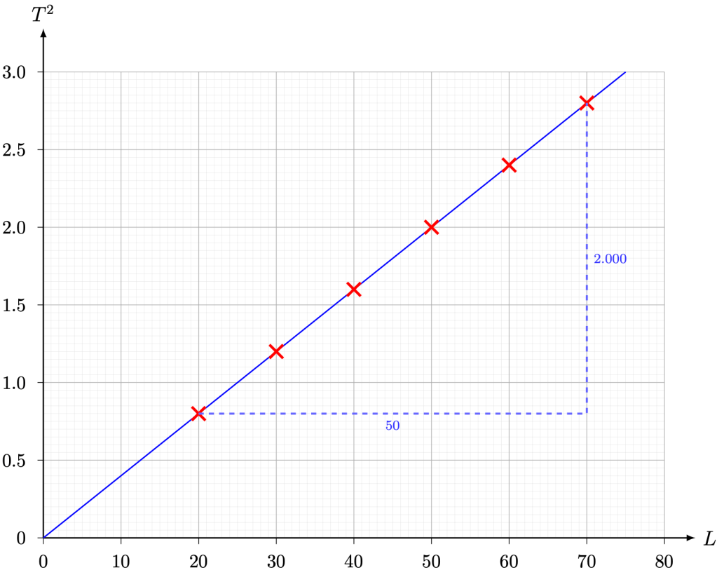


 and
and  . Hence, estimate the value of f correct to 3 significant figures.


 against t. Hence, estimate the values of k and x0.
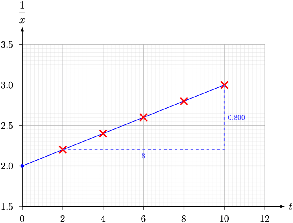

 and
and  , we have
  .
. and
and  , we have
  .
.
 , then there exists some nonzero
  such that
  . Since
  ,
,

 , there exists
  such that
  . As specific instances,


 . By Problem 4,
 . Calculating the percentage change yields

 . By Problem 4,
 . Calculating the percentage change yields
 , we have
 . By Problem 4,
 . Calculating the relative change yields

 equals the constant
  and
and  such that

 is an integer and
  , we have
  .
.