Using our basic ideas of probability, let’s discuss a simple yet deep problem in probability theory, which laid the foundational ideas for quantitative finance; the gambler’s ruin.
Disclaimer. This page does not promote or encourage online gambling in any form. The information presented here is for educational purposes only.
The gambler’s ruin can be formulated simply. Let 


- You start with
.
- On each turn
- If the coin lands ‘Head’, you win
, so that
.
- If the coin lands ‘Tail’, you lose
.
- If the coin lands ‘Head’, you win
- The game ends at the first time
when
.
Suppose the simplest case 


Example 1. What is the probability that 

Solution. By definition, 

In Example 1, getting a ‘Head’ yields 


Remark 1. The fun really begins when we vary our setup. In fancy quantitative financial language, we call 


Now let’s set 

Example 2. What is the probability that 

Solution. Since we are dealing with multiple coin tosses, it gets exponentially difficult to intuit the solution. Since this process involves consecutive time steps, we can visualise its process using a probability tree diagram. As its name suggests, it is a diagram that resembles a tree that is described using probabilities.
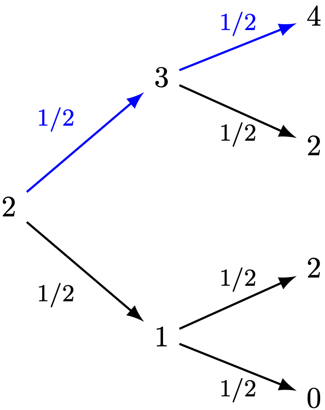
The number 

We note that 


Therefore,

Similarly, 

the required probability is

Now suppose 
Example 3. Evaluate 
Solution. We extend our probability tree diagram as follows.
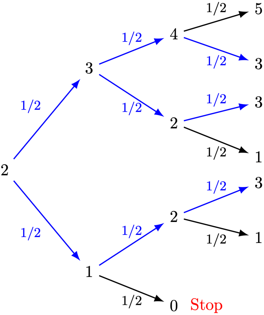
This time, the “total number of possibilities” argument fails. Why? Because the game ended for wealth trajectory 
Nevertheless, we can still solve the problem. Each coin toss doesn’t impact the next one, so that the sample space

contains outcomes that all share the same probability. For instance,

In fancier language, we say that the coin tosses are independent of each other. This logic holds no matter the coin toss; letting 

In particular, each path with length 


Therefore, 
Remark 2. When presenting our work, you do not need to be so long-winded as per this writeup. As long as you communicate your thought process through your calculation, you can obtain full credit.
Example 4. How would the answer in Example 3 change if we are working with a biased coin with probability 


Solution. We modify our probability tree diagram as follows.
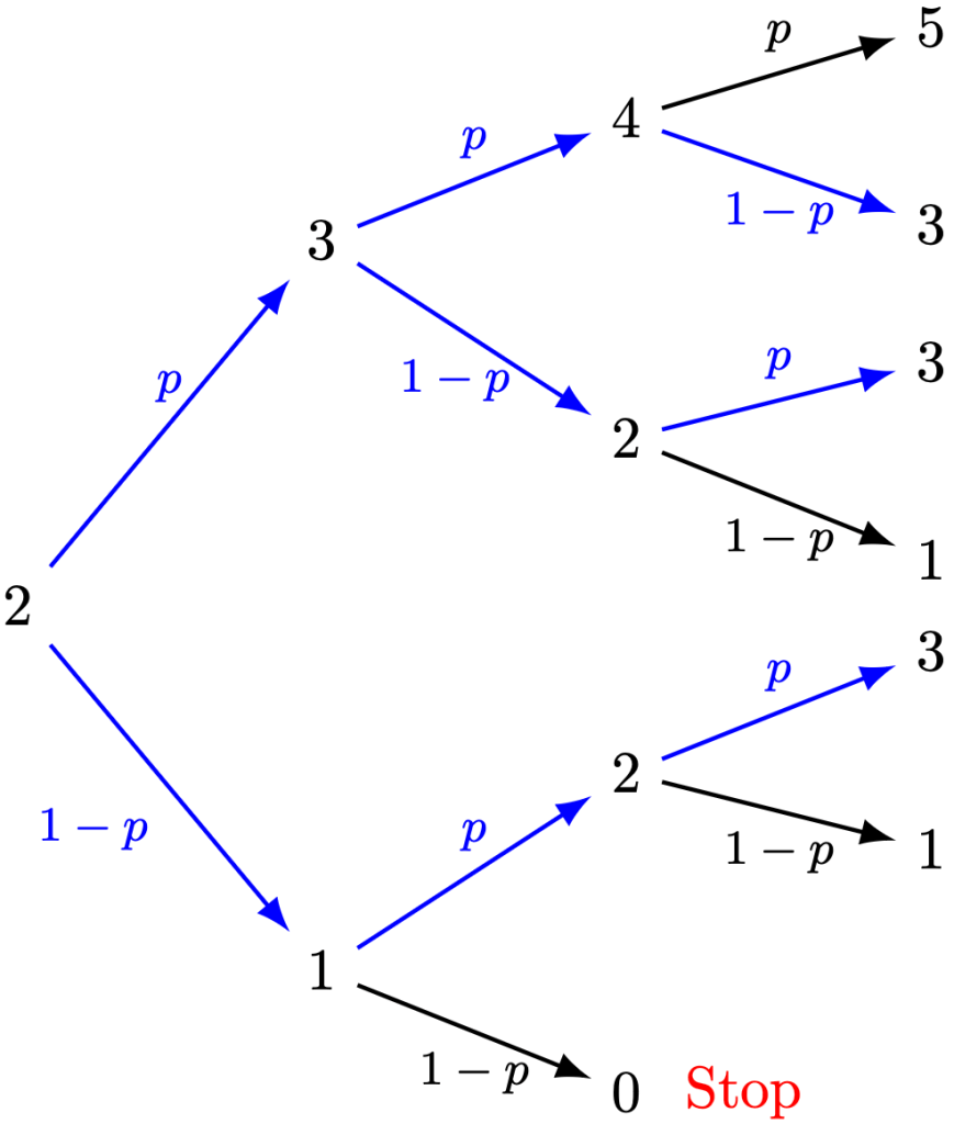
The visual is basically the same, and we would follow the same trajectories
However, each step has as slightly different probability to compute:

Since all paths are distinct, and turn out to have the same probabilities, we can sum the probabilities up as follows:

Remark 3. This process can be generalised to what is known in probability and statistics as the binomial distribution. The multiplication procedure is known as the multiplication principle, used to calculate probabilities of in-sequence events. The addition procedure is known as the addition principle, used to calculate probabilities of disjoint events.
Example 5. Toss a biased coin with probability
Solution. Draw the probability tree diagram as follows.
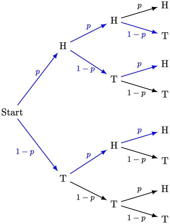
By following the chosen trajectories, the required probability is

The answer in Example 5 matches the answer in Example 4. This observation should not be a surprise—the wealth trajectories in Example 4 are directly determined by the coin tosses in Example 5 and vice versa.
Remark 3. These example suggest that studying probability is less inherently about the underlying random process, but more so about the distributions of the possible outcomes.
Example 6. You have 4 black socks and 6 white socks in your drawer. You choose two socks at random, without replacement (obviously). What is the probability that you get two socks of the same color?
Proof. We draw the following probability tree diagram.
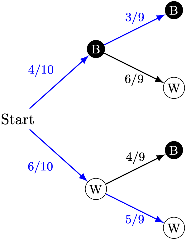
Notice that if the first sock chosen is black, then the probability of the second sock chosen would change (since there is one less black sock present). Following the two routes of matching-coloured socks, the required probability is given by

Of course, the coin toss is one of the simpler examples to begin our discussions on probability theory. Another common toy that we use to discuss probabilities would be that of dice. A fair six-sided die has 6 faces: 1, 2, 3, 4, 5, 6, each occurring with equal probability 
Example 7. Roll two fair die simultaneously. Assume that the outcomes of the dice are independent. What is the probability that the numbers sum to 

Solution. Let 


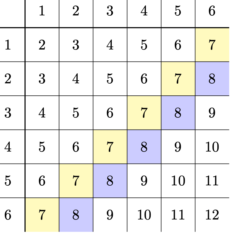
For example, if 


Among all possible sums, 7 has the largest number of cells, namely 6. Therefore, the required integer is 

Remark 4. If the dice are unfair, we can still manually compute 

one after another for 


If there is one topic that I insist on discussing applications, it would most certainly be probability. I do think it is a good idea to illustrate probability in the real world. To do that, I’ll need to discuss matrices, which also happens to be our final topic in O-Level mathematics. Of course, we can extend these ideas at great length into the study of stochastic processes and Markov chains, but let’s just touch base with some simple examples to augment our understanding.
—Joel Kindiak, 18 Mar 26, 1539H

Leave a comment