Comparing the entries of the matrices on both sides yields and .
Define and .
Problem 3. Show that .
(Click for Solution)
Solution. We observe that . By Problem 1,
Similarly, . Therefore, .
Define .
Problem 4. Evaluate . Hence, if , construct a matrix with the property that
(Click for Solution)
Solution. Using the multiplication in Problem 3 but setting and ,
If , then either or , so that . Therefore,
Denoting , define , so that
By Problem 3, .
Problem 5. Determine the two possible matrices such that
(Click for Solution)
Solution. Write . Using the multiplication in Problem 3 with and ,
Therefore,
Grouping the terms together,
Using Problem 2,
Using the second equation, either or . If , then substituting into the first equation,
However, this equation has discriminant, and so there are no real roots to the equation, a contradiction.
Therefore, we must have . Substituting into the first equation again,
Therefore, . Hence, the two possible matrices for are
We can condense them to the expression .
Remark 1. By denoting and , we have created a model for the complex numbers, where by Problem 1. In particular, numbers of the form are called purely imaginary. The solution to Problem 5 would then look like
The letter ‘z‘ is used to denote a complex number by convention. Furthermore, the calculation motivates the (somewhat debatable) notation . For more information, see this post.
Let’s drink some milk tea! Consider the three milk tea chains in Singapore: Chagee, Koi, and LiHo. (There are many others, so please experiment with these other chains if you wish.)
Let denote the proportion of the population that drinks Chagee, Koi, and LiHo respectively at time , measured in months. For simplicity, assume that customers are exclusive and loyal—Chagee drinkers do not drink from Koi and vice versa.
Before Chagee came on the scene, the milk tea scene was mostly split between Koi and LiHo, so that . Let’s suppose that 50% of the population drank Koi and 50% of the population drank LiHo at time t, measured in months, so that and . Since LiHo is newer than Koi, suppose the following changes happen after each month:
2% of Koi drinkers switch to LiHo,
1% of LiHo drinkers switch to Koi.
Example 1. At the end of the first month, what proportion of the population would be Koi drinkers?
Solution. We can represent these changes using the following diagram. Arrows once again represent similar ideas as they do in probability tree diagrams: the arrow from Koi to LiHo with label 0.02 means that 0.02 of Koi drinkers switch to LiHo.
Recall that denotes the proportion of the population that drinks Chagee, Koi, and LiHo respectively at the end of month . Since Chagee has not yet existed in the Singapore market, . Now is determined by two quantities:
the 98% of Koi customers who remained loyal to Koi,
the 1% of LiHo customers who switched to Koi.
Therefore,
Similarly,
Since , we can substitute them into both equations and obtain as our desired answer:
Indeed, Koi lost a small amount of its market share, as predicted.
Now suppose the proportion of drinkers as per Example 1. For reasons that will become apparent later, let’s denote the market shares as vectors:
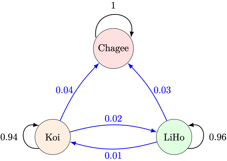
Due to aggressive social media marketing by Chagee’s youthful team, suppose at the end of every month, the following changes happen after each month:
4% of Koi drinkers switch to Chagee,
3% of LiHo drinkers switch to Chagee.
All Chagee drinkers keep drinking Chagee.
Question 1. At the end of the second month, what proportion of the population would be Chagee drinkers?
We can represent these changes using the following diagram, now including Chagee in our calculations.
Using similar analysis to Example 1, we write out the following three equations:
Use vector notation to simplify our work:
At this point in time, all we need to do is to substitute , , and to obtain our answer (as an exercise, check that ). But what if we wanted to re-use this information to answer more sophisticated questions? Wouldn’t it be nice to condense this information even further?
Remark 1. The setups we gave are specific kinds of Markov chains and more generally, stochastic processes, an model of describing sequences of random variables that satisfy sufficiently nice probability properties.
We can think of the three vectors as the “ingredients” needed that produce our result, while the numbers denote a “recipe” in combining these ingredients. To that end, mathematicians and statisticians stack the ingredients side-by-side as a matrix, and place the “recipe” vector on the right-hand side:
This is, in fact, the essential origin-story of the matrix. It wasn’t a-priori defined as a table of numbers equipped with some out-of-the-blue calculations; it was simply a summary of changing data!
Remark2. Notice that the notion of a 3-dimensional vector just arose from our problem setup. In the physical world, we can still visualise 3 dimensions, but more complicated setups would require the use of -dimensional vectors, where . In these settings, physical intuition fails, but we can still reason about them through formalised mathematical definitions.
Definition 1. An matrix is an -dimensional vector. For example, we have the following matrix :
An matrix is a collection of vectors, each of them -dimensional, placed beside each other:
For example, we have the following matrix and matrix :
Furthermore, given an -dimensional vector , we define the expression to mean
Define the zero matrix by .
Example 2. Evaluate the expression
giving your answer in terms of a 2-dimensional vector.
Solution. Using Definition 1,
Remark 2. The expression in Example 2, being contrived, doesn’t represent any particular real-world example. However, its calculations are identical to that of the milk tea example (which is, itself, not entirely faithful to reality, but simplified for analogous purposes).
Example 3. Given an matrix , how many dimensions must the vector have so that makes sense?
Solution. Write
where each is an -dimensional vector. Since has “ingredients” that combined with “recipe” vector gives the “dishes” , our “recipe” vector should have components. That is, should be -dimensional.
If we could add vectors, could we add matrices? The real question is, why not? Consider the two expressions below:
Let’s expand both terms using the recipe-ingredient analogy:
Now let’s add both sides of the equation together:
where we consolidated our calculations using the recipe-ingredient analogy again. Therefore, it is reasonable to define
so that for any 3-dimensional vector ,
A similar thought process works for multiplying a matrix by a number (i.e. scalar multiplication) and matrix subtraction.
Definition 2. Let and be matrices. Define matrix addition “ingredient-wise” by
so that for any -dimensional vector , .
Similarly, given any real number , define scalar multiplication “ingredient-wise” by
so that for any -dimensional vector , .
In particular, define , and .
Example 4. Show that .
Solution. By Definition 2 and its implications,
Example 5. Evaluate the following expressions:
Solution. Using Definition 2,
Theorem 1. Given matrices and scalars , the following matrix properties hold:
,
,
,
,
,
,
,
.
Proof. Left as a tedious (but ultimately meaningful) exercise.
How might we multiply two matrices together? Consider the expression
Using the ingredient-recipe analogy, the matrix on the right-hand side has two recipes, not one. Therefore, we can think of the expression as cooking two dishes; this is our definition of matrix multiplication:
And we know how to compute the “dishes” and using Definition 1.
Example 6. Given an matrix , what must the size of the matrix be in order for the expression to make sense?
Solution. Write
By definition,
In order for each to make sense, by Example 3, each should be -dimensional. Since there are columns in , the size of must be , where can be any positive integer.
Example 7. Evaluate the expression
Solution. Applying Definition 1 to each column,
Combining the results,
Example 8. Given , evaluate .
Solution. By definition,
Applying Definition 1 to each column,
Combining the results,
Example 9. Show that
where for any ,
Solution. By the ingredient-recipe analogy, the -th column would be given by
Expanding the left-hand side,
Therefore,
In particular, by comparing the -th row,
Remark 3.Example 9 is the conventional definition of matrix multiplication, which I have avoided to define a priori since it seems contrived and miscellaneous, rather than the current presentation which shows how matrix multiplication is a necessary consequence of the information-preserving properties that we aimed to achieve.
And that’s all for matrices! Matrices, at the O-level is simply a tool to summarise systems of linear equations. All of its arithmetical properties simply arise from preserving said information. When put together with vectors, we get the all-encompassing study of linear algebra. Here are some further questions you might think about involving matrices and vectors.
Consider the matrix and the vector .
What vector would satisfy the equation ?
Is it possible to divide by ?
Are there numbers and vectors such that ?
Is it possible to compute in an efficient manner?
Does the equation have at least some best approximation?
These questions turn out to be basic problems in undergraduate linear algebra, and are used all the time in applied STEM, like physics, engineering, economics, and finance.
Remark 1. This writeup is a fresh writeup because somehow, and tragically, the original post got permanently deleted.
Our goal is to answer a simple question: how do we solve the cubic equation? Namely, given constants with , if we know that the real number satisfies the equation
how might we determine the possible values of ? Firstly, we had better be sure that this equation can be solved, and the power of is the ticket to why that holds.
Theorem 1. The cubic equation has at least one real solution.
Proof. Omitted; we can achieve this result by adapting the proof of Theorem 2 in this post.
There is a general “cubic” formula, but we shall work with special cases in which the root in Theorem 1 could be obtained with trial-and-error.
We abbreviate the left-hand side by . Then, we call a root of the polynomial if and only if . In particular,
Lemma 1. For any real number ,
Proof. Firstly, we expand the right-hand side to obtain
Then we replace with to obtain
Lemma 2. For any real number , there exist unique real constants such that
Proof. Making the substitutions and applying Lemma 1,
where we set and .
Lemma 2 paves the way for the special case of the remainder and factor theorems—the general case follows a factorisation of by generalising the argument in Lemma 1.
Theorem 1. Given any real number , there exists a unique polynomial and a unique real number , called the remainder, such that
Furthermore, —this result is known as the remainder theorem. Finally, this remainder equals zero if and only if is a root of —this result is known as the factor theorem. In this case, we say that is a factor of the polynomial .
Proof. By Lemma 2,
yielding and .
For uniqueness, set to obtain . Then
For , dividing by yields . For a more complete argument regarding uniqueness, see this post.
While we have discussed the result in an overly abstract manner, perhaps it is worth elucidating the theory with an example.
Example 1. Solve the cubic equation .
Solution. Define . By almost-obvious observation,
Therefore, by the factor theorem, is a factor of . Hence, there exist constants such that
Comparing the coefficients of and the constant term respectively, and . Comparing the coefficient of ,
Therefore,
Since , we must have either
In the former, . In the latter, we solve using the quadratic formula: first compute the discriminant . Then
Solution. We leave a similar-to-Example 1 solution left as an exercise to the reader. By taking advantage of the similar numbers, we divide the equation by :
Now make the substitution to obtain a rather suspect equation:
By re-arranging the terms, we obtain the exact same equation as that in Example 1, just with different letters:
Therefore, by Example 1, we have or . Since , the former yields , and the latter takes a bit more work by rationalising the denominator:
As mentioned, there is a cubic formula, and it also turns out there is a quartic formula, i.e. a general formula to solve the equation
where . How about a quintic formula?
The answer turns out to be no, and requires a study of generalised algebra to prove.
For now, we deal with more contained higher powers, of the form , called binomials.
Using our basic ideas of probability, let’s discuss a simple yet deep problem in probability theory, which laid the foundational ideas for quantitative finance; the gambler’s ruin.
Disclaimer. This page does not promote or encourage online gambling in any form. The information presented here is for educational purposes only.
The gambler’s ruin can be formulated simply. Let be pre-determined integers and denote your wealth, in dollars, at time :
You start with .
On each turn , you toss a fair coin.
If the coin lands ‘Head’, you win , so that .
If the coin lands ‘Tail’, you lose , so that .
The game ends at the first time when .
Suppose the simplest case , , and .
Example 1. What is the probability that ? What about the result ?
Solution. By definition, . Since the coin is fair,
In Example 1, getting a ‘Head’ yields , and getting a ‘Tail’ yields . No matter the outcome, we have . Furthermore, . Therefore, rather trivially, the game ends at time .
Remark 1. The fun really begins when we vary our setup. In fancy quantitative financial language, we call a stopping time for the time series process. The quantity models our stop loss, models our capital, and models our take profit. The coin being fair is a simplistic starting point for discussion—in the real world the price movements are far less predictable than we would hope for.
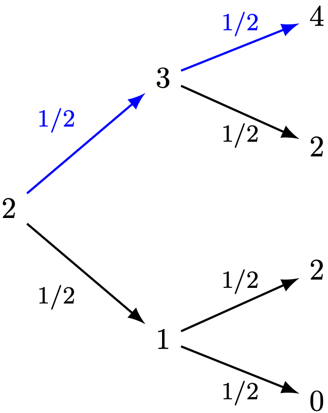
Now let’s set , , and .
Example 2. What is the probability that ? How about ?
Solution. Since we are dealing with multiple coin tosses, it gets exponentially difficult to intuit the solution. Since this process involves consecutive time steps, we can visualise its process using a probability tree diagram. As its name suggests, it is a diagram that resembles a tree that is described using probabilities.
The number on the lines denote the probability that the wealth increases or decreases by $1 respectively. There are four possible paths that the wealth can take, and they all occur with equal probability. Denote the sample space by the wealth evolutions:
We note that corresponds to wealth evolutions of the form . Since the only outcome when this result takes place is , we write
Therefore,
Similarly, corresponds to wealth evolutions of the form . Since there now are two such wealth evolutions, so that
,
the required probability is
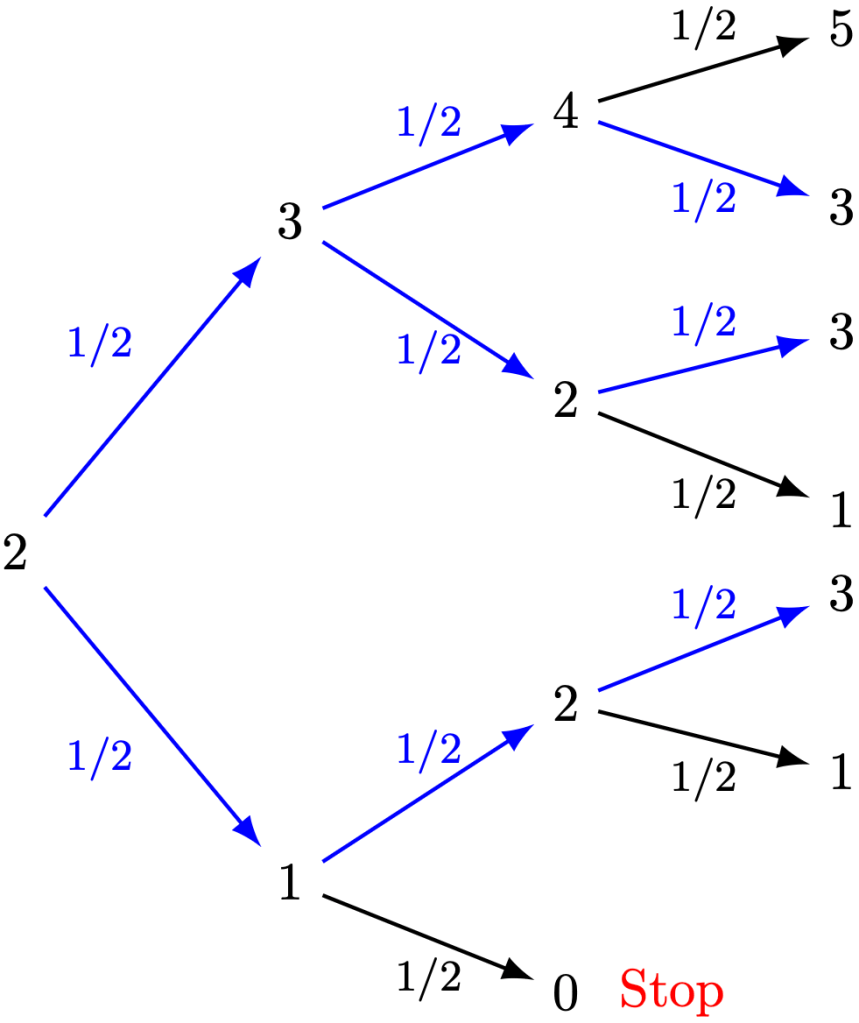
Now suppose , , .
Example 3. Evaluate .
Solution. We extend our probability tree diagram as follows.
This time, the “total number of possibilities” argument fails. Why? Because the game ended for wealth trajectory .
Nevertheless, we can still solve the problem. Each coin toss doesn’t impact the next one, so that the sample space
contains outcomes that all share the same probability. For instance,
In fancier language, we say that the coin tosses are independent of each other. This logic holds no matter the coin toss; letting denote individual coin tosses, we have
In particular, each path with length will automatically have a probability of of occurring. Notice that there are three paths that get us to :
Therefore, .
Remark 2. When presenting our work, you do not need to be so long-winded as per this writeup. As long as you communicate your thought process through your calculation, you can obtain full credit.
Example 4. How would the answer in Example 3 change if we are working with a biased coin with probability ? That is, and . Give your answer in terms of .
Solution. We modify our probability tree diagram as follows.
The visual is basically the same, and we would follow the same trajectories
However, each step has as slightly different probability to compute:
Since all paths are distinct, and turn out to have the same probabilities, we can sum the probabilities up as follows:
Remark 3. This process can be generalised to what is known in probability and statistics as the binomial distribution. The multiplication procedure is known as the multiplication principle, used to calculate probabilities of in-sequence events. The addition procedure is known as the addition principle, used to calculate probabilities of disjoint events.
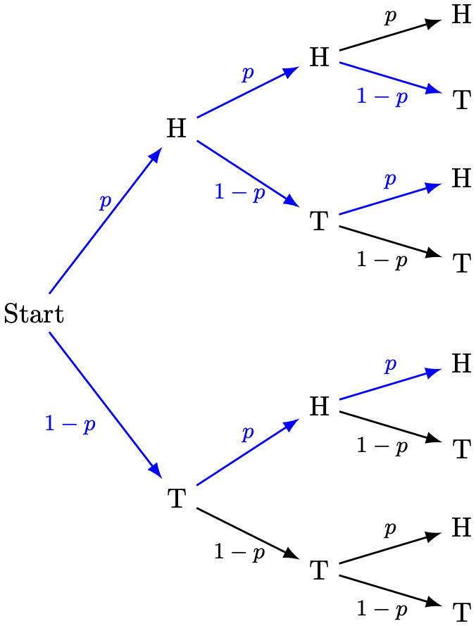
Example 5. Toss a biased coin with probability three times. What is the probability that you get two ‘Heads’? What do you notice?
Solution. Draw the probability tree diagram as follows.
By following the chosen trajectories, the required probability is
The answer in Example 5 matches the answer in Example 4. This observation should not be a surprise—the wealth trajectories in Example 4 are directly determined by the coin tosses in Example 5 and vice versa.
Remark 3. These example suggest that studying probability is less inherently about the underlying random process, but more so about the distributions of the possible outcomes.
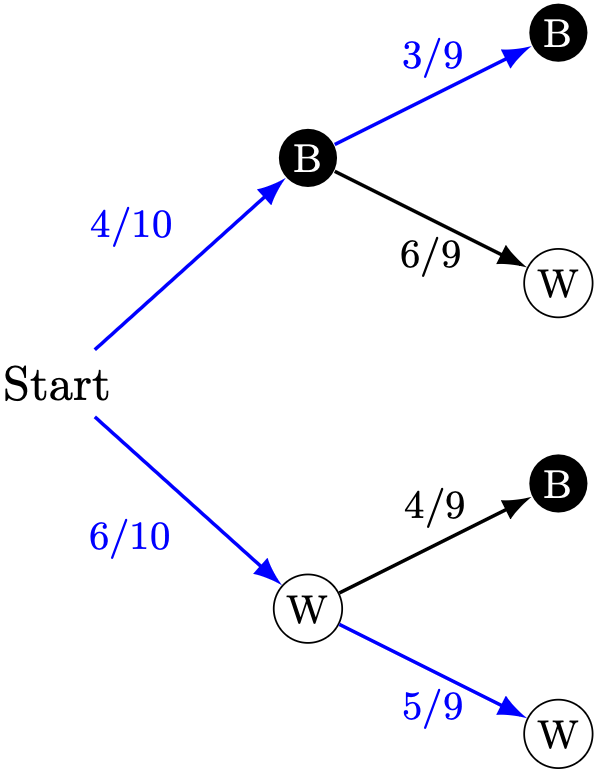
Example 6. You have 4 black socks and 6 white socks in your drawer. You choose two socks at random, without replacement (obviously). What is the probability that you get two socks of the same color?
Proof. We draw the following probability tree diagram.
Notice that if the first sock chosen is black, then the probability of the second sock chosen would change (since there is one less black sock present). Following the two routes of matching-coloured socks, the required probability is given by
Of course, the coin toss is one of the simpler examples to begin our discussions on probability theory. Another common toy that we use to discuss probabilities would be that of dice. A fair six-sided die has 6 faces: 1, 2, 3, 4, 5, 6, each occurring with equal probability .
Example 7. Roll two fair die simultaneously. Assume that the outcomes of the dice are independent. What is the probability that the numbers sum to ? Which integer is the most probability sum?
Solution. Let denote the outcome of the first die and denote the outcome of the second die. We want to evaluate . We can illustrate the outcome of sums using the possibility diagam below.
For example, if and , then . Since the dice are independent, each cell has a probability of , which also agrees intuitively with the possibility diagram. Since there are 5 cells whose sum yields 8, the required probability is
Among all possible sums, 7 has the largest number of cells, namely 6. Therefore, the required integer is , and in fact,
Remark 4. If the dice are unfair, we can still manually compute by adding up the separate cases
one after another for . Of course if or , then . This process is known as taking the discrete convolution between two probability mass functions.
If there is one topic that I insist on discussing applications, it would most certainly be probability. I do think it is a good idea to illustrate probability in the real world. To do that, I’ll need to discuss matrices, which also happens to be our final topic in O-Level mathematics. Of course, we can extend these ideas at great length into the study of stochastic processes and Markov chains, but let’s just touch base with some simple examples to augment our understanding.
Previously, we looked at evaluating and summarising data. Data is mostly randomly generated, though not necessarily in a purely unpredictable manner, by chance. It is of our interest, therefore, to now turn to games of chance.
Consider a fair 6-sided die with possible values (plural: dice). We collect these outcomes into a set, defined , and collect sub-collections of these outcomes also as sets.
Example 1. Write down the sub-collection of even-numbered outcomes of the die.
Solution. Since the even-numbered outcomes of the die are , the required subset is .
Definition 1. Let be sets. We write:
if the two sets have exactly the same elements,
and call a subset of if is a sub-collection of ,
if is not a subset of .
For instance, in Example 1, we have . We can illustrate this relationship using a Venn diagram.
Therefore, we will use sets in order to model chance. However, sets alone don’t get at the full picture. We also need to quantify certainty. Intuitively, since there are 3 even numbers in the set , then the probability that we roll an even number on the die should be . We formalise this idea using sets.
For any (finite) set , let denote the number of elements in the set. For instance, and .
Definition 2. Let be a set, which we usually call the universal set of discourse. Given , define the uniformprobability of by
Using the language of Definition 2, the probability of rolling an even number on the die is displayed as
Denote for simplicity, because we are lazy. Recall that .
Remark 1. Observe that , and . Furthermore, some education systems denote the universal set by the following alternate notation and use them in their assessments: . In the spirit of learning set-formulated probability theory, we will not follow such practice in these blog posts.
Example 2. What is the probability that we would roll a multiple of ?
Solution. The multiples of are described by the subset . Therefore, the required probability is
Example 3. What is the probability that we would roll an even multiple of ?
Solution. The even numbers are given by the subset , and the multiples of are given by the subset . The common number is , and therefore the subset of that contains all even multiples of is . Therefore, the required probability is
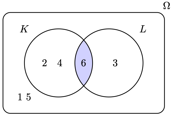
To capture the idea of “common elements”, we use the notion of the intersection. We can illustrate this common-ness using another Venn diagram.
In order to do that, we need to introduce the idea of “membership”.
Definition 3. Let be a set. We write to mean that belongs to . In this case, we say that is an element of . We write to mean that does not belong to .
For instance, if , then and . Furthermore, we can write in set-builder notation:
Definition 4. Let be subsets of . We call the sub-collection of common elements the intersection of and . Formally, we define this intersection by
For example .
Example 4. What is the probability that we would roll a number that is both odd and even?
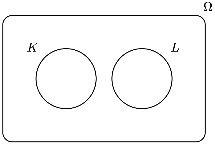
Solution. The subset of odd numbers is and the subset of even numbers is . There…are no numbers in that belong to both subsets. The required subset is empty: . In the language of Definition 4,
Therefore, the required probability is
Remark 2. We denote , motivated by the observation . Furthermore, we say that are mutually disjoint since .
Example 5. What is the probability that we would roll a number that is either even or a multiple of ?
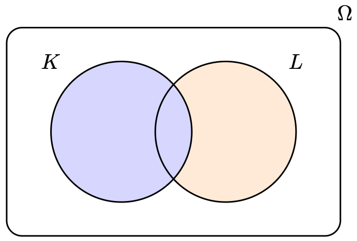
Solution. If we require a number to be at least one of these criterion, we allow it to be taken from either of the subsets or , then the desired subset would be . We can illustrate this “collaboration” using another Venn diagram.
Therefore, the required probability is
Definition 5. Let be subsets of . We call the sub-collection of “collaborated” elements the union of and . Formally, we define this union by
For example .
Example 6. What is the probability that we would roll a number that is not a multiple of ?
Solution. By accepting all elements of that are not multiples of , the desired subset is . We can visualise this subset, once again, using a Venn diagram.
Therefore, the required probability is
Definition 6. For any , define the complement of by
For example, .
At this point, alarm bells should ring, since by Remark 1 and Example 2,
Furthermore, we notice that
That is, we can add probabilities of unions of mutually exclusive subsets.
Theorem 1. Let be mutually disjoint subsets of . Then
Proof. Since are mutually disjoint, every element in belongs either to and not, or and not.
Therefore, must equal , and hence,
Remark 3. This property holds for any number of mutually disjoint subsets:
whenever each whenever . This result is called the (finite or countable) additivity property of probability.
Corollary 1. Given ,
Proof. By definition, and . By Remark 1 and Theorem 1,
Therefore, .
Remark 4. In particular, so that
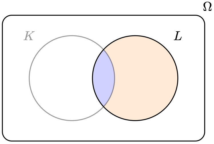
Example 7. Given subsets , not necessarily disjoint, show that
Solution. Consider the Venn diagram below for illustrative purposes.
Given , there are two non-overlapping cases:
and .
Denoting for brevity,
By Theorem 1,
On the other hand, we observe that given , either or . Refer to the zoomed-in Venn diagram below.
Therefore,
By Theorem 1 again,
Making the subject of the equation,
Therefore, we use set notation to describe our intuitive notions of probability. We can formalise these ideas with far more advanced tools, but we shall relegate that rabbit hole as an exercise for the keen reader. We keep these ideas simple for now.
Next time, we solve some simple problems involving probability.
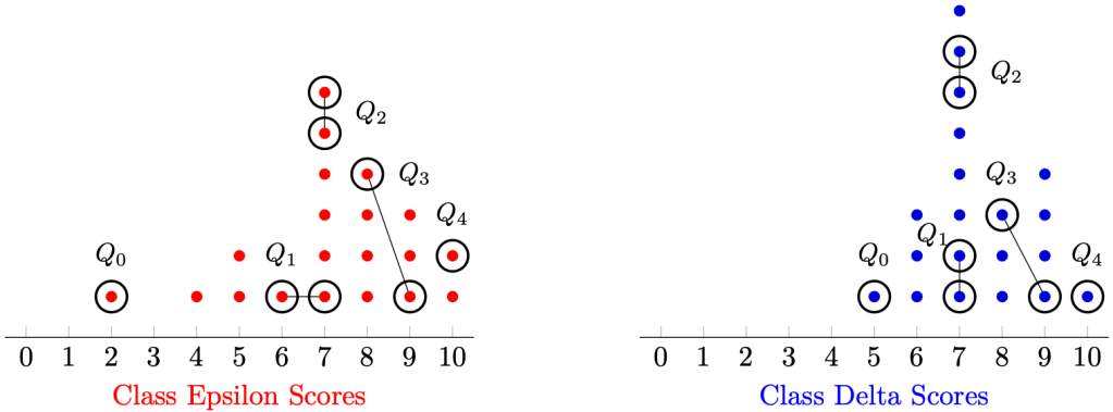
In the mock data below, the scores of a class test (total score: 10) for two classes, each with 20 students, are plotted in the dot diagram below.
Which of the two classes did better?
This question is vague. What do we mean by “better”? We would usually like to make this decision according to some summarised data (i.e. statistics). Previously, we have learned that the most computationally convenient statistic to describe the centre of the data is the mean, given by the formula
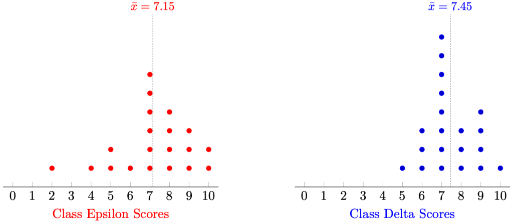
Running the calculations, Class Epsilon has mean 7.15 and Class Delta has mean 7.45.
Using the mean as our measurement of aura, we might conclude that Class Epsilon is stronger than Class Delta in the exam.
But you can—and should—object: Class Delta has not just one, but two students who scored full marks! Furthermore, we notice that it seems like Class Delta’s mean score is lowered due to some poor-performing outliers. That is, Class Delta has a larger spread of data when compared to the data of Class Epsilon.
The tool that statisticians use is called the standard deviation. The intuitive idea is that we want to find the average of the deviations of the data points from the sample mean. To ensure that this calculation is mathematically convenient, we square these deviations.
Definition 1. For each data point , determine its squared deviation by . The sample variance is then simply defined by , and the standarddeviation is defined by .
Remark 1. This squared-deviation idea is responsible for linear regression—a fundamental algorithm in modern machine learning.
Theorem 1. The formula to compute the standard deviation of the sample is given by
Proof. Denote the data set by . Compute the squared deviations by
By definition, . Therefore,
Dividing by on all sides,
Taking square roots,
Remark 2. If we had a collection of paired data , we can compute the sample covariance between the data set and by
Observe that . In this regard, the sample covariance generalises the sample variance. Here, the covariance measures the extent of connection between the two data sets.
Example 1. Using the standard deviation as the measure of spread, Class Epsilon has a standard deviation of approximately 2.01 and Class Delta has a standard deviation of approximately 1.28.
Since the latter is larger, Class Epsilon has a larger spread of scores than Class Delta.
In layperson’s terms, the scores of students in Class Epsilon are more “bunched” together, and thus we can say that the students in Class Epsilon perform more consistently than the students in Class Delta.
However, we should object to this conclusion once again: why did we use the mean and the standard deviation? These statistics are sensitive to outlier data, be it exceedingly high-performing students or exceedingly low-performing students. Why not use the median?
We can, and should: in this case, Class Epsilon has a median score of 7 and Class Delta has a median score of 7. Not helpful. How would we measure the spread of the data?
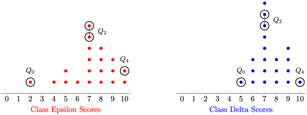
Definition 2. Sort the dataset into a non-decreasing order
Denote the:
minimum by
the median by ,
the maximum by ,
Define the range of the data set by .
Obviously, and . If is even, then
If is odd, then .
Remark 3. The latter Q denotes the word ‘quartile’. Therefore, the minimum can be thought of as the “zeroth” quartile, the median as the second quartile, and the maximum as the fourth quartile.
Example 2. The range in Class Epsilon is 8 and the range in Class Delta is 5. Therefore, there is larger spread in Class Epsilon than Class Delta.
But you should, once again, object to this conclusion. This measure of spread accounts for the vast outliers! Can we obtain a measure of spread that disregards outliers, just like how the median disregards outliers?
Definition 3. Suppose a data set where is odd, and it has a median of . Define:
the lower quartile by the median of the data set ,
the upper quartile by the median of the data set ,
the interquartile range by .
Question 1. How would you define the interquartile range if were even?
Example 3. By definition,
Class Epsilon has a lower quartile of 6.5 and upper quartile of 8.5, and hence, an interquartile range of 2.
Class Delta has a lower quartile of 7 and upper quartile of 8.5, and hence, an interquartile range of 1.5.
Since the former is larger than the latter, we conclude that there is larger spread in Class Epsilon than Class Delta.
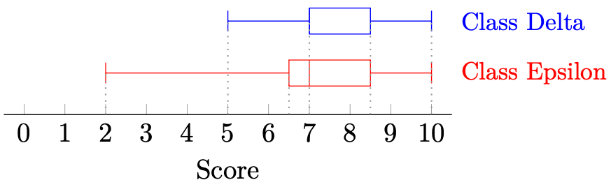
We can visualise the ordered information using box-and-whisker diagrams. The endpoints denote the minimum and maximum, the box denotes the interquartile range, and the centre line denotes the median. We can plot both box-and-whisker diagrams below.
Therefore, the box-and-whisker diagram helps us visualise the data in a sufficiently meaningful manner. The distinct vertical lines denote respectively.
Remark 4. For Class Delta, , explaining why it appears to have only four lines instead of the expected five.
I have one more idea to discuss—large data sets. So far, our class sizes are small, just 20 sample points. However, if we consider all of the students in the school, we would need to deal with large data sets, say 1000. Suppose also the total score of the assessment is 100, rather than 10. How do we interpret such data? We can use a cumulative frequency diagram.
The -axis denotes the number of data points, with . The -axis denotes the score of the assessment, out of 100. The curve plots the following information: lies on the curve precisely when students scored at most marks in the assessment.
Remark 5. Cumulative frequency diagrams, being discrete, tend to be more jagged than what we see displayed. Nevertheless, this smooth approximation turns out to be mostly accurate relative to our original data.
Example 4. Estimate the median, range, and interquartile range of the data. Use your estimates to represent the data using a box-and-whisker diagram.
Solution. It is clear that and , so that the range is 100. We estimate as follows.
Therefore, we estimate the median to be 69 marks, and the interquartile range to be 18 marks.
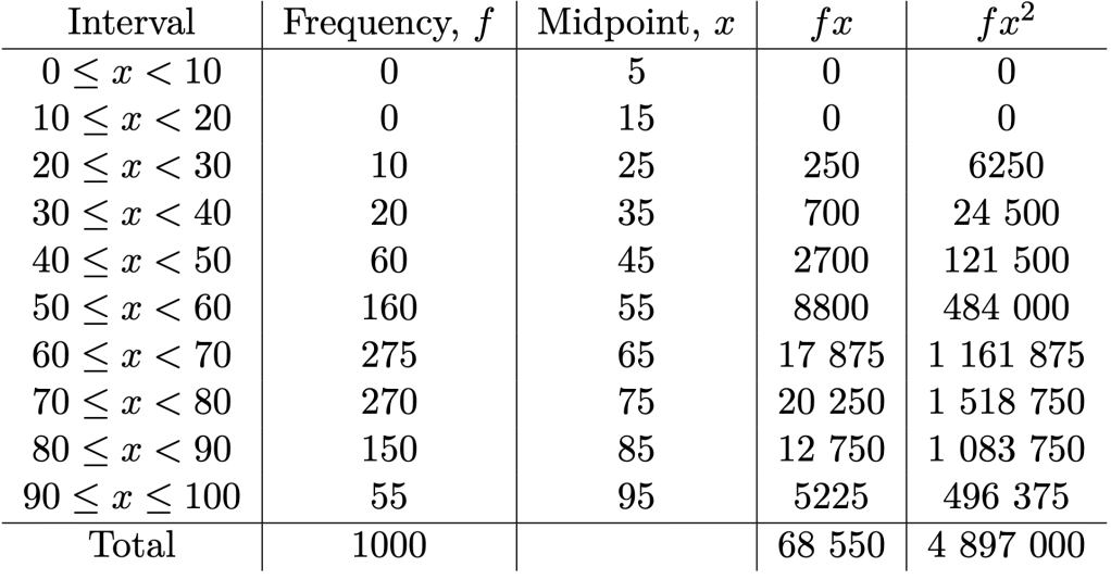
Example 5. Using intervals of 10 marks each, estimate the mean and the standard deviation of the data.
Solution. We leave it as an exercise to tabulate the following summarised data.
In particular,
Therefore, we estimate the mean of the data to be
and by Theorem 1, the standard deviation of the data to be
Remark 6. In the era of Microsoft Excel and Python, software can compute means and standard deviations of large datasets without using the grouped data approach. They can handle millions of computations—we can’t.
Would you still object? In the spirit of inquiry and scepticism, why not? However, I think my job here is done—I have introduced the key calculations required in secondary school statistics!
Just for fun, for those of you curious about quantitative finance, where you use mathematics and statistics to possibly win the stock market or even the cryptocurrency market. Individuals working in these fields, called quants, use the Sharpe ratio, defined by , to determine the riskiness of an asset. Another measure of riskiness known as the mean-variance, defined by , helps quants optimise the proportion of their assets in order to minimise risk.
Finally, for Singaporeans who (or whose parents) remember the notion of a t-score in the high-stakes Primary School Leaving Examinations (PSLE), the student’s final score for a particular subject is computed using the formula
and these numbers are summed over the four subjects: English, Mother Tongue, Mathematics, and Science. My PSLE score was 242—make of that as you will. Contrary to popular expectation, I did *not* get A* for Mathematics due to less-than-academically-important reasons.
All of these statistical analyses arise from random phenomenon, and are general grasps of otherwise un-graspable realities. But can we at least quantify such uncertainty? Our attempt at doing so is probability theory, and we will visit this idea briefly the next time.
In this post, we will explore some basic notions in quantitative finance.
More specifically, buying and selling stocks.
Suppose 1 unit of a stock KMATH costs $1 at time t = 0. Assume negligible trading fees.
Problem 1. At time t = 0, you buy 200 units of KMATH. What is the value of your position?
(Click for Solution)
Solution. The value of units of KMATH is
Problem 2. Suppose at time t = 1, the price per unit of KMATH increased by 10%. What is the value of your position at t = 1?
(Click for Solution)
Solution. The value of the position has increased by , that is,
Therefore, the position has a new value of
Alternate Solution. If the initial position has a value of and the price increased by a percentage of , then the position increases by the value
Therefore, the position would have a new value of
In particular, setting and
in Problem 2 yields a new value of
Problem 3. Suppose at time t = 2, the price per unit of KMATH decreased by 10%. What is the overall change in your position from t = 0 to t = 2? How about its overall percentage change? Is your position in a profit or a loss?
(Click for Solution)
Solution. We will use the calculation in Remark 1. Let
denote the percentage decrease of the price per unit of KMATH from to .
By Remark 1, the new position at is . Therefore, the new position at has a value of
Substituting , the new position has a value of
The overall percentage change is
Since the percentage change is negative, our position currently sits in a loss.
Problem 4. For any positive integer n, let rn denote the percentage change in your position from t = n – 1 to t = n. Show that the overall percentage change between t = 0 and t = n is calculated by
1 + r = (1 + r1) × (1 + r2) × … × (1 + rn).
(Click for Solution)
Solution. Let denote the value of the position at time . Applying the alternate solution in Problem 2 repeatedly,
On the other hand, denoting the overall percentage change by , we have
Equating the two sides,
Dividing by on both sides yields the desired result:
Problem 5. What is the minimum percentage increase of the price per unit of KMATH from t = 2 to t = 3 required for you to not incur loss?
(Click for Solution)
Solution. Let denote the required percentage increase of the price per unit of KMATH from to . By Problem 3, the overall percentage change is given by
Substituting and , since and , we can divide on both sides to obtain
Subtracting by on both sides,
Since we do not want to incur loss, the overall percentage change must be non-negative, that is to say, :
In particular, we need more than increase in order to compensate for an overall decrease of .
Problem 1. Illustrate the two vectors in the diagram below.
Show that the angle between is given by
(Click for Solution)
Solution. Observe that
Using the law of cosines,
Expanding the display on the left-hand side by Pythagoras’ theorem,
Comparing both sides of the expression ,
as required.
Remark 1. The left-hand side is called the dot product of two vectors, defined by
Then the result of Question 1 reduces to the dot product equation
Let denote a real constant and denote another two-dimensional vector.
Problem 2. Using Remark 1, show that the following equations always hold:
.
.
.
.
.
(Click for Solution)
Solution. Write and . The first result is almost immediate since are real numbers:
For the second result
Furthermore,
Hence, . Similarly, . Hence .
The third property is straightforward:
Recall that . Then
Define . Then the fifth property is immediate:
Problem 3. Explain why . Deduce the following:
.
.
.
.
.
(Click for Solution)
Solution. Using Remark 1 and Pythagoras’ theorem,
Therefore, we obtain the properties rather straightforwardly:
with equality if and only if . Next,
The fourth property, known as the Cauchy-Schwarz inequality, follows from Problem 1 and the observation that :
The fifth property follows from the fourth:
and taking square roots on both sides.
Problem 4. Define . Show that the following hold:
.
.
.
.
(Click for Solution)
Solution. The results in Problem 4 comes from Problem 3:
then
Furthermore,
and
Remark 2. In the language of linear algebra, Remark 1 and Problem 2 defines a “multiplication” on the set of two-dimensional vectors, turning it into a realinner product space. Problem 3 show that inner product spaces are normed spaces (in that two-dimensional vectors have lengths or norms), while Problem 4 shows that normed spaces are metric spaces (i.e. the notion of distance is a reasonable one).
Problem 5. Given that the point lies on the line , show that any other point lies on the line if and only if
(Click for Solution)
Solution. Since lies on the line, we have
The point lies on the line if and only if
Subtracting the equations yields the equation
On the other hand,
Then lies on the line if and only if the right-hand side equals , that is,
Remark 3.Problem 5 generalises to an -dimensional hyperplane: Given that the point lies on the -dimensional hyperplane with equation
any other point lies on the hyperplane if and only if


 and
and  as follows:
 .
.
 be real numbers.
 and
and  .
.
 and
and  and
and  .
. .
. . By Problem 1,
 . Therefore,
  .
. . Hence, if
  , construct a matrix
  with the property that
 and
and  ,
,
 or
or  , so that
  . Therefore,
 , define
  , so that
 .
. such that
 ,
,


 or
or  . If
. If 
 , and so there are no real roots to the equation, a contradiction.
 . Hence, the two possible matrices for
  are
are
 .
. and
and  , we have created a model for the complex numbers
  , where
  by Problem 1. In particular, numbers of the form
  are called purely imaginary. The solution to Problem 5 would then look like
 . For more information, see
 denote the proportion of the population that drinks Chagee, Koi, and LiHo respectively at time
  , measured in months. For simplicity, assume that customers are exclusive and loyal—Chagee drinkers do not drink from Koi and vice versa.
 . Let’s suppose that 50% of the population drank Koi and 50% of the population drank LiHo at time t, measured in months, so that
  and
and  . Since LiHo is newer than Koi, suppose the following changes happen after each month:
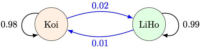
 denotes the proportion of the population that drinks Chagee, Koi, and LiHo respectively at the end of month
  . Since Chagee has not yet existed in the Singapore market,
  . Now
. Now  is determined by two quantities:

 , we can substitute them into both equations and obtain


 , and
, and  to obtain our answer (as an exercise, check that
  ). But what if we wanted to re-use this information to answer more sophisticated questions? Wouldn’t it be nice to condense this information even further?
 -dimensional vectors, where
  . In these settings, physical intuition fails, but we can still reason about them through formalised mathematical definitions.
  matrix is an
  -dimensional vector. For example, we have the following
  matrix
  :
:
 matrix is a collection of
 matrix
  and
and  matrix
  :
:
 , we define the expression
  to mean
 .
.

 have so that
  makes sense?
 is an
is an 


 ,
,
 and
and  be
be 
 .
. , define scalar multiplication “ingredient-wise” by
 .
. , and
, and  .
. .
.


 matrices
  and scalars
  , the following matrix properties hold:
 ,
, ,
, ,
, ,
, ,
, ,
, ,
, .
.

 and
and  using Definition 1.
 to make sense?

 to make sense, by Example 3, each
  should be
  columns in
  , where


 , evaluate
  .
.


 ,
,
 -th column would be given by


 -th row,
 .
. would satisfy the equation
  ?
? and vectors
  ?
? in an efficient manner?
 satisfies the equation
 is the ticket to why that holds.
 has at least one real solution.
 . Then, we call
  if and only if
  . In particular,


 to obtain
 such that
![\begin{aligned} f(x) - f(\alpha) &= (a x^3 + b x^2 + c x + d) - (a \alpha^3 + b \alpha^2 + c \alpha + d) \\ &= a(x^3 - \alpha^3) + b(x^2-\alpha^2) + c(x-\alpha) + d(1-1) \\ &= a(x-\alpha)(x^2 + \alpha x + \alpha^2) + b(x-\alpha)(x+\alpha) + c(x-\alpha) \\ &= (x-\alpha)( a (x^2 + \alpha x + \alpha^2) + b (x+\alpha) + c ) \\ &= a(x-\alpha)\left[ (x^2 + \alpha x + \alpha^2) + \frac ba (x+ \alpha) + \frac ca \right] \\ &= a(x-\alpha)\left[ x^2 + \alpha x + \alpha^2 + \frac ba x+ \frac ba \alpha + \frac ca \right] \\ &= a(x-\alpha)\left[ x^2 + \left( \alpha + \frac ba \right) x + \left( \alpha^2 + \frac ba \alpha + \frac ca \right) \right] \\ &= a(x-\alpha) ( x^2 + k x + m ), \end{aligned}](https://s0.wp.com/latex.php?latex=%5Cbegin%7Baligned%7D+f%28x%29+-+f%28%5Calpha%29+%26%3D+%28a+x%5E3+%2B+b+x%5E2+%2B+c+x+%2B+d%29+-+%28a+%5Calpha%5E3+%2B+b+%5Calpha%5E2+%2B+c+%5Calpha+%2B+d%29+%5C%5C+%26%3D+a%28x%5E3+-+%5Calpha%5E3%29+%2B+b%28x%5E2-%5Calpha%5E2%29+%2B+c%28x-%5Calpha%29+%2B+d%281-1%29+%5C%5C+%26%3D+a%28x-%5Calpha%29%28x%5E2+%2B+%5Calpha+x+%2B+%5Calpha%5E2%29+%2B+b%28x-%5Calpha%29%28x%2B%5Calpha%29+%2B+c%28x-%5Calpha%29+%5C%5C+%26%3D+%28x-%5Calpha%29%28+a+%28x%5E2+%2B+%5Calpha+x+%2B+%5Calpha%5E2%29+%2B+b+%28x%2B%5Calpha%29+%2B+c++%29+%5C%5C+%26%3D+a%28x-%5Calpha%29%5Cleft%5B++%28x%5E2+%2B+%5Calpha+x+%2B+%5Calpha%5E2%29+%2B+%5Cfrac+ba+%28x%2B+%5Calpha%29+%2B+%5Cfrac+ca+%5Cright%5D+%5C%5C+%26%3D+a%28x-%5Calpha%29%5Cleft%5B++x%5E2+%2B+%5Calpha+x+%2B+%5Calpha%5E2+%2B+%5Cfrac+ba+x%2B+%5Cfrac+ba+%5Calpha+%2B+%5Cfrac+ca+%5Cright%5D+%5C%5C+%26%3D+a%28x-%5Calpha%29%5Cleft%5B++x%5E2+%2B+%5Cleft%28+%5Calpha+%2B+%5Cfrac+ba+%5Cright%29+x+%2B+%5Cleft%28+%5Calpha%5E2+%2B+%5Cfrac+ba+%5Calpha+%2B+%5Cfrac+ca+%5Cright%29+%5Cright%5D+%5C%5C+%26%3D+a%28x-%5Calpha%29+%28++x%5E2+%2B+k+x+%2B+m+%29%2C+%5Cend%7Baligned%7D&bg=ffffff&fg=000&s=0&c=20201002)
 and
and  .
. by generalising the argument in Lemma 1.
 and a unique real number
  , called the remainder, such that
 —this result is known as the remainder theorem. Finally, this remainder equals zero if and only if
  is a factor of the polynomial
 and
and  . Then
 , dividing by
  . For a more complete argument regarding uniqueness, see
  .
. . By almost-obvious observation,
 is a factor of
  such that
 and the constant term respectively,
  and
and  . Comparing the coefficient of
  ,
,


 . In the latter, we solve using the
  . Then
 .
. .
.
 to obtain a rather suspect equation:

 or
or  . Since
  , the former yields
  , and the latter takes a bit more work by rationalising the denominator:

 . How about a quintic formula?
 , called
  be pre-determined integers and
  denote your wealth, in dollars, at time
  .
. , so that
  .
. .
. when
when  .
. ,
,  , and
, and  .
. ? What about the result
  ?
? . Since the coin is fair,
 , and getting a ‘Tail’ yields
  . No matter the outcome, we have
  . Furthermore,
  . Therefore, rather trivially, the game ends at time
  .
. models our stop loss,
  models our capital, and
  models our take profit. The coin being fair is a simplistic starting point for discussion—in the real world the price movements are far less predictable than we would hope for.
 , and
, and  .
. ? How about
  ?
?
 on the lines denote the probability that the wealth increases or decreases by $1 respectively. There are four possible paths that the wealth can take, and they all occur with equal probability. Denote the sample space by the wealth evolutions:
 . Since the only outcome when this result takes place is
  , we write

 . Since there now are two such wealth evolutions, so that
 ,
,
 .
. .
.
 .
.

 denote individual coin tosses, we have
 of occurring. Notice that there are three paths that get us to
  :
:
 .
. ? That is,
  and
and  . Give your answer in terms of
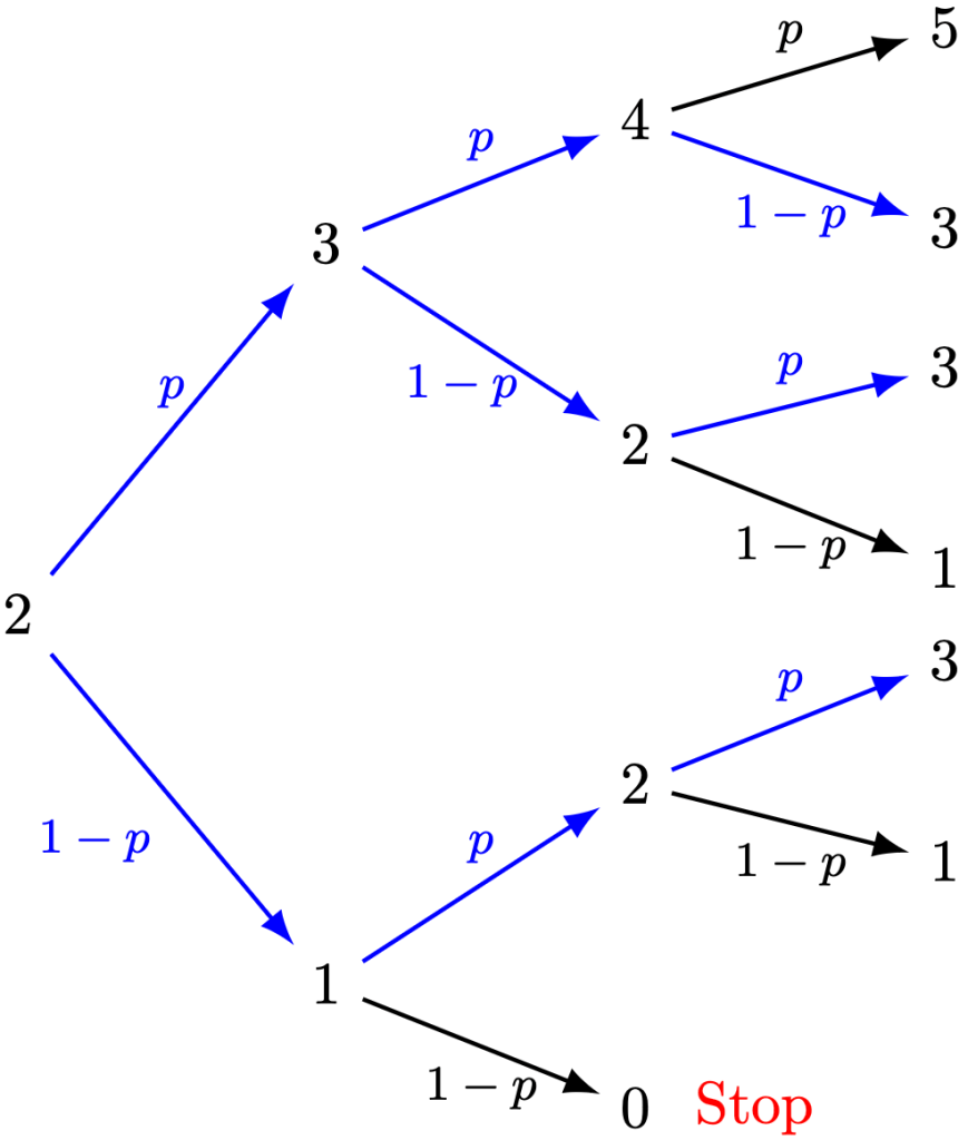


 .
. ? Which integer
  denote the outcome of the first die and
  denote the outcome of the second die. We want to evaluate
  . We can illustrate the outcome of sums using the possibility diagam below.
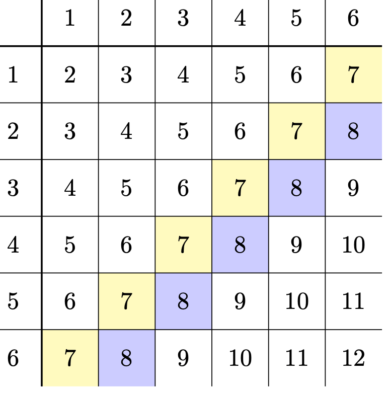
 and
and  , then
  . Since the dice are independent, each cell has a probability of
  , which also agrees intuitively with the possibility diagram. Since there are 5 cells whose sum yields 8, the required probability is
 , and in fact,
 by adding up the separate cases
 . Of course if
  or
or  , then
  . This process is known as taking the discrete convolution between two probability mass functions.
 (plural: dice). We collect these outcomes into a set, defined
  , and collect sub-collections of these outcomes also as sets.
 , the required subset is
  .
. be sets. We write:
 if the two sets have exactly the same elements,
 and call
  a subset of
  if
if  . We can illustrate this relationship using a Venn diagram.
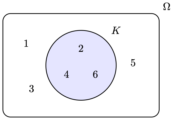
 . We formalise this idea using sets.
 denote the number of elements in the set. For instance,
  and
and  .
. be a set, which we usually call the universal set of discourse. Given
  , define the uniform probability of

 for simplicity, because we are lazy. Recall that
  .
. , and
, and  . Furthermore, some education systems denote the universal set by the following alternate notation and use them in their assessments:
  . In the spirit of learning set-formulated probability theory, we will not follow such practice in these blog posts.
 . Therefore, the required probability is
 , and the multiples of
  . The common number is
  , and therefore the subset of
  . Therefore, the required probability is
 to mean that
  to mean that
  , then
  and
and  . Furthermore, we can write
 of common elements the intersection of
 .
. and the subset of even numbers is
  . In the language of Definition 4,

 , motivated by the observation
  . Furthermore, we say that
  .
.
 . We can illustrate this “collaboration” using another Venn diagram.
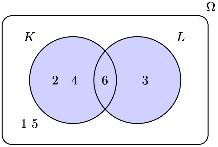


 .
. that are not multiples of
  . We can visualise this subset, once again, using a Venn diagram.
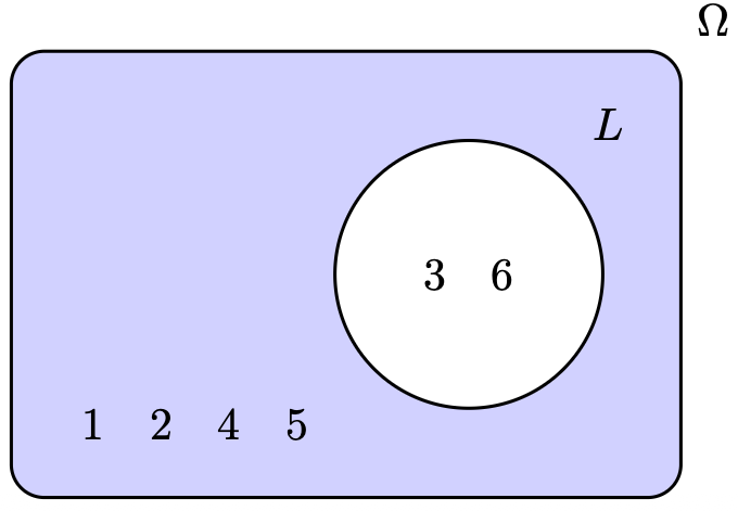


 .
.


 belongs either to
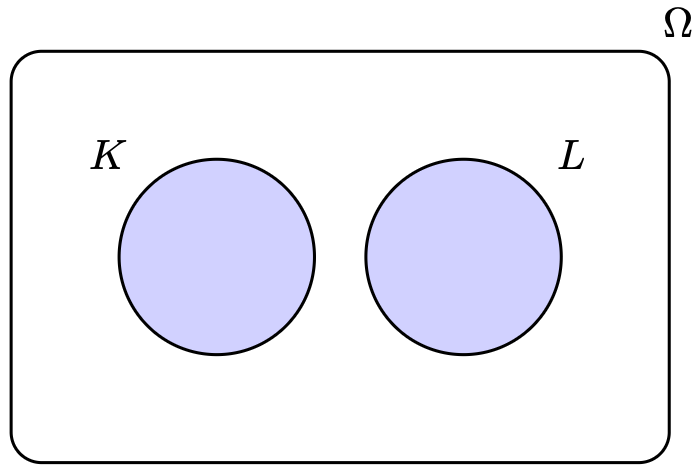
 must equal
  , and hence,

 whenever
  . This result is called the (finite or countable) additivity property of probability.
 and
and  . By Remark 1 and Theorem 1,
 .
. so that

 , there are two non-overlapping cases:
 and
and  for brevity,


 the subject of the equation,
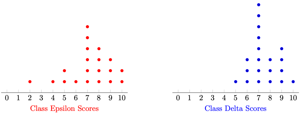

 . The sample variance
  is then simply defined by
  , and the standard deviation is defined by
  .
. of the sample is given by
 . Compute the squared deviations by
 . Therefore,


 , we can compute the sample covariance
  between the data set
  and
and  by
by
 . In this regard, the sample covariance generalises the sample variance. Here, the covariance measures the extent of connection between the two data sets.
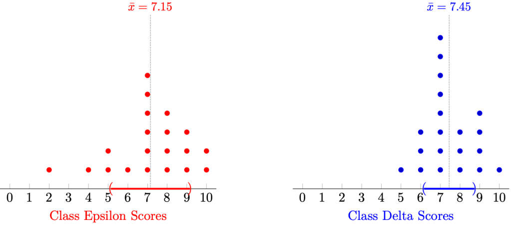


 ,
, ,
, .
. and
and  . If
. If 
 .
. 
 . Define:
 by the median of the data set
  ,
, by the median of the data set
  ,
, .
.
 respectively.
 , explaining why it appears to have only four lines instead of the expected five.
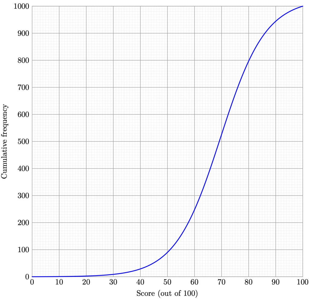
 -axis denotes the number of data points, with
  . The
. The  plots the following information:
  lies on the curve precisely when
  and
and  , so that the range is 100. We estimate
  as follows.
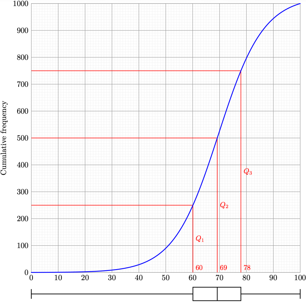


 , to determine the riskiness of an asset. Another measure of riskiness known as the mean-variance, defined by
  , helps quants optimise the proportion of their assets in order to minimise risk.
 units of KMATH is
 , that is,

 and the price increased by a percentage of
  , then the position increases by the value

 and
and


 to
to  .
. . Therefore, the new position at
 , the new position has a value of

 denote the value of the position at time
  . Applying the alternate solution in Problem 2 repeatedly,


 on both sides yields the desired result:
 denote the required percentage increase of the price per unit of KMATH from
  . By Problem 3, the overall percentage change
 and
and  , since
  and
and  , we can divide on both sides to obtain

 :
:
 increase in order to compensate for an overall decrease of
  , where
 ,
, ,
,
 . Using the extended definitions of
  , for
, for 
 or
or
 -periodic:


 and
and  ,
,
 or
or  , where
  , where
 , for
, for 
 or
or
 , where
 , for
, for 
 or
or
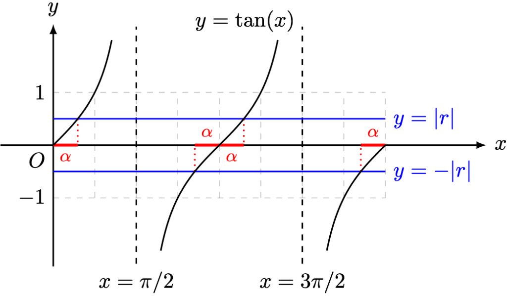
 , solve the equation
  , where
  .
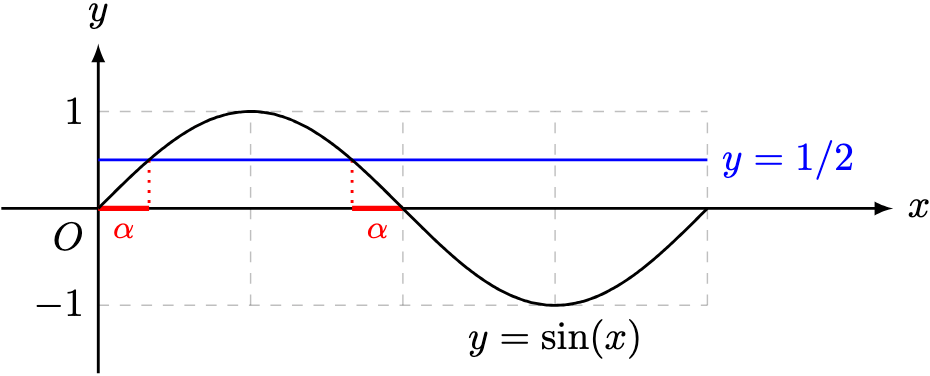
. . Using special angles, we recall that for
  ,
,

 or
or 
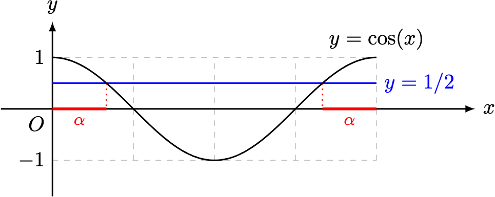
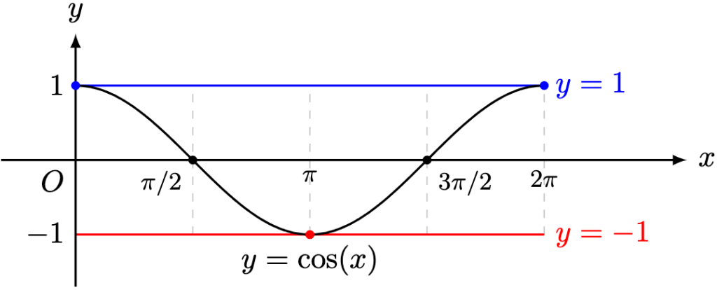
 . Using special angles, we recall that for

 .
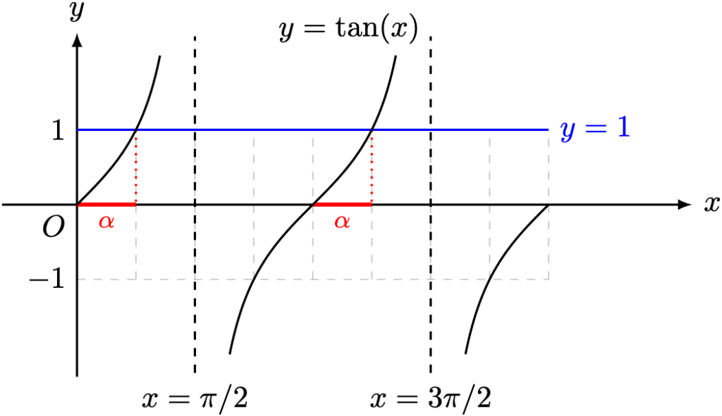
. . Using the same equations as the case for
  , or
, or .
. .
. , where
  is an integer.
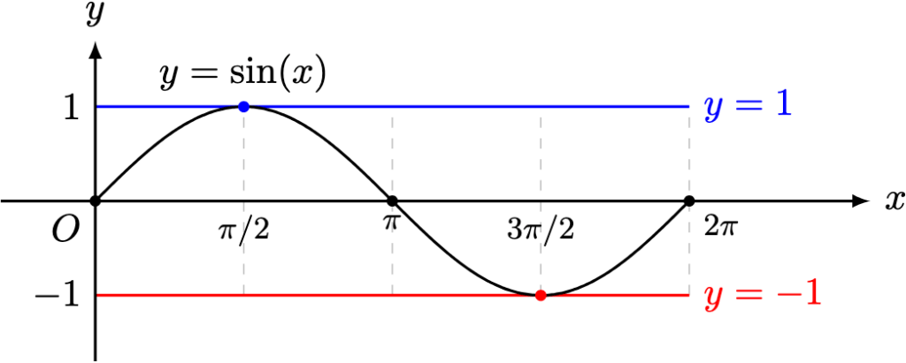
 , where
 ,
, ,
, .
.
 . Define
  such that

 , then only the first two equations work:
  .
. :
:  , then only the last two equations work:
  .
.


 .
. by Problem 5.
 .
.

 in terms of
 .
. .
.
 , the solutions for
  , the candidate solutions in the domain


 , the candidate solutions in the domain

 , the candidate solutions in the domain

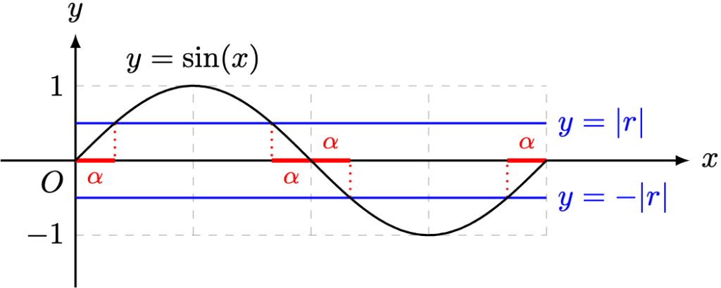
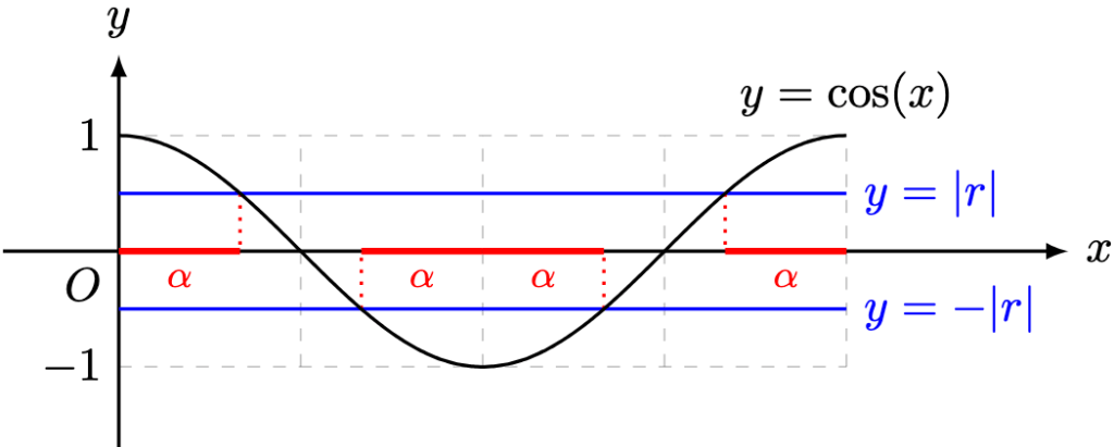
 for
for  so that
  . To solve the equation
 ,
,

 to obtain all solutions in
 for
for  .
.
 :
:
 or
or  . In the former,
 , this equation has no solutions. Therefore,
 in the diagram below.
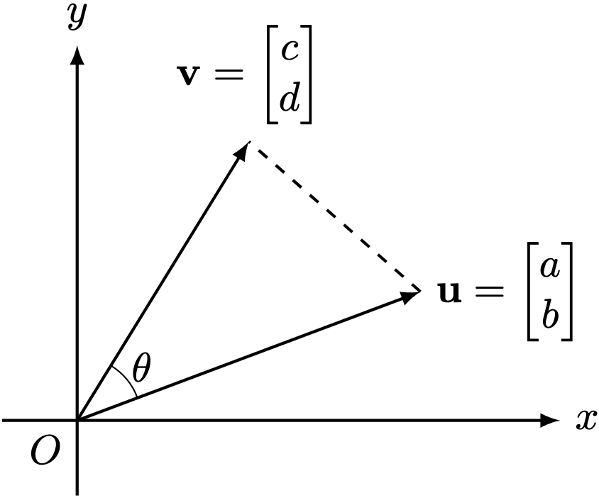
 between
  is given by


 ,
,


 denote another two-dimensional vector.
 .
. .
. .
. .
. .
. and
and  . The first result is almost immediate since
  are real numbers:


 . Similarly,
  . Hence
  .
.
 . Then
 . Then the fifth property is immediate:
 . Deduce the following:
 .
. .
. .
. .
. .
.

 . Next,
 :
:

 . Show that the following hold:
 .
. .
. .
. .
.


 lies on the line
  , show that any other point


 , that is,
 -dimensional hyperplane: Given that the point
  lies on the
 lies on the hyperplane if and only if
