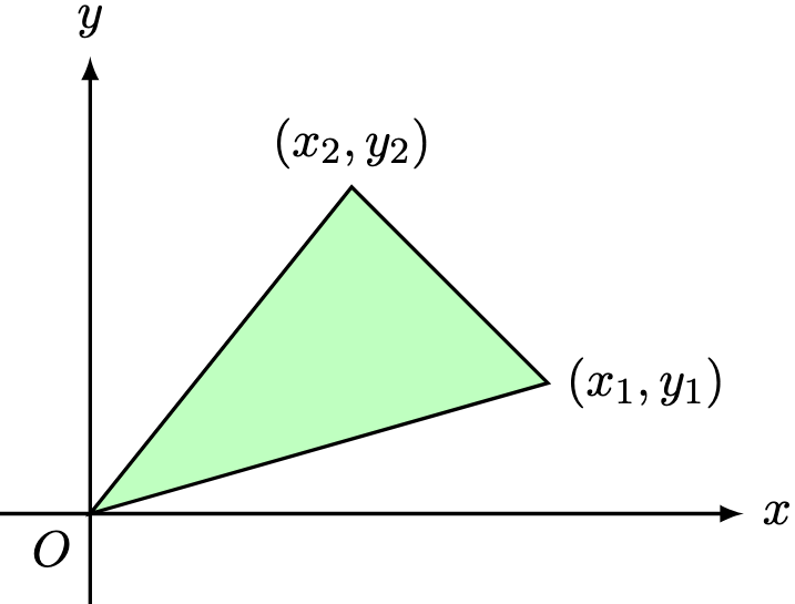
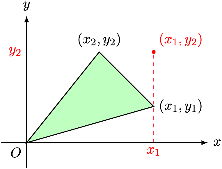
Solution. Add dashed lines to draw in “phantom” triangles.
We subtract the area of the three smaller triangles from the larger rectangle:
Remark 1. There are many other kinds of triangles, but with enough patience, they can all be shown to yield the same area formula.
Definition 1. Define
In particular, the area of the triangle in Problem 1 can be written as .
Problem 2. Show that . In particular,
(Click for Solution)
Solution. By definition,
Remark 1. In particular, a polygon is said to have positive orientation if its coordinates are traversed in anti-clockwise direction, and have negative orientation if its coordinates are traversed in clock-wise direction.
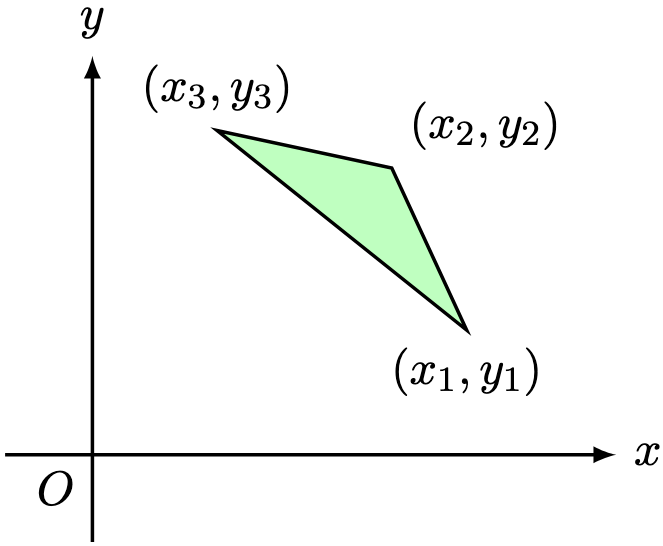
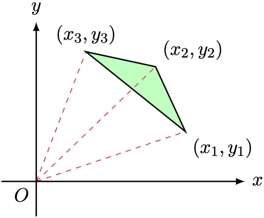
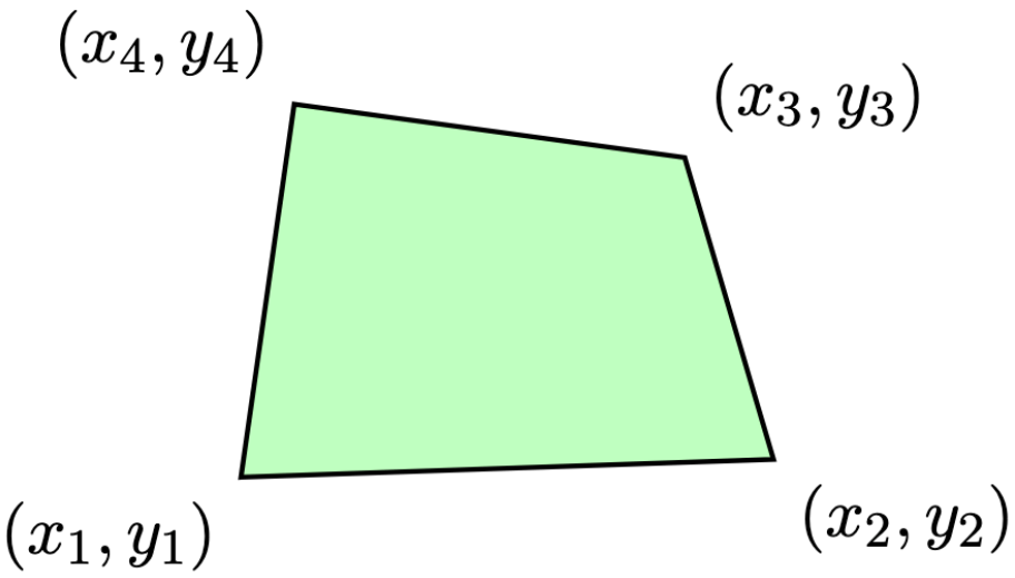
Problem 3. Consider the triangle below with positive orientation.
Show that the triangle has area
(Click for Solution)
Solution. Draw some “phantom” triangles:
Denote the area of the triangle by . By Problem 1,
By Problem 2,
Remark 2. In a similar manner, for triangles with other orientations, as long as the vertices are traversed in an anti-clockwise direction, we still recover the same formula as in Problem 3.
Definition 2. Make the notation
This notation is commonly referred to as the shoelace formula. In particular, the area in Problem 3 can be expressed as
Problem 4. Show that
(Click for Solution)
Solution. Patiently expand the right-hand side:
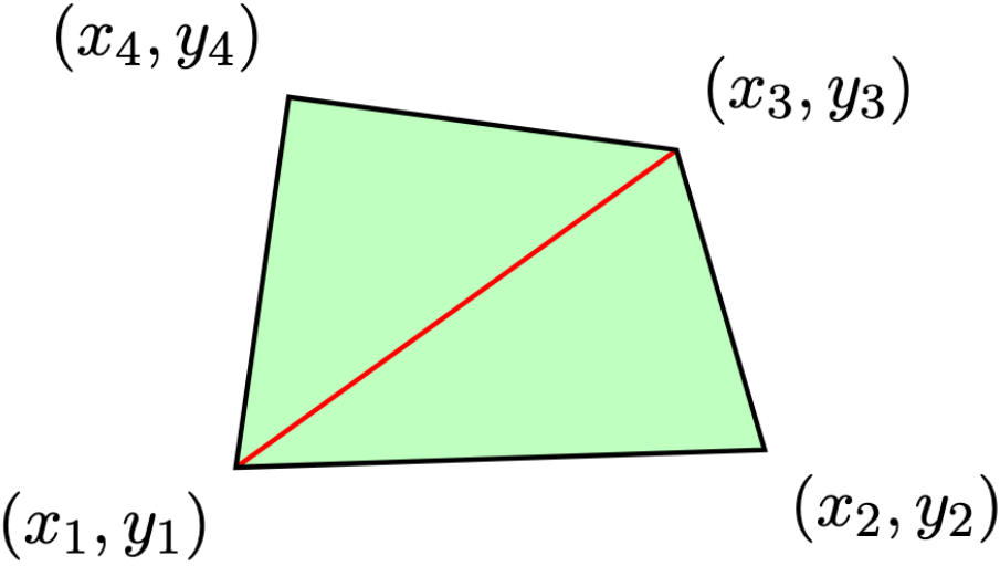
Problem 5. Consider the quadrilateral below.
Show that the quadrilateral has area
(Click for Solution)
Solution. Connect to .
The quadrilateral consists of two triangles, and therefore its area is given by the sum of both triangles, whose formulas are given by Problem 4:
where the comes from Problem 2. Multiplying both sides by yields the formula
Remark 2. Using mathematical induction and the same strategy in Problem 5, the signed area of an -gon with vertices
can be shown to equal
Furthermore, this quantity is positive if the vertices are traversed in an anti-clockwise direction and negative if the vertices are traversed in a clockwise direction.
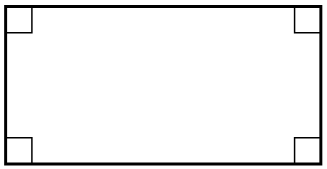
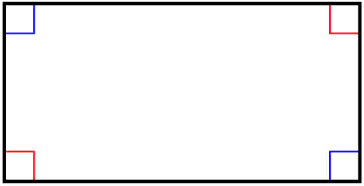
Definition 1. A quadrilateral is a four-sided shape.
For example, a rectangle is a quadrilateral whose internal angles are all .
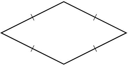
Definition 2. A rhombus is a quadrilateral with equal side lengths.
Problem 1. Show that a quadrilateral is a square if and only if it is both a rectangle and a rhombus.
(Click for Solution)
Solution. Suppose a quadrilateral is both a rectangle and a rhombus.
As a rectangle, all of its angles are .
As a rhombus, all of its side lengths are equal.
Therefore, it must be a square.
Trivial.
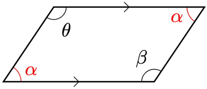
Definition 3. A parallelogram is a quadrilateral with two pairs of parallel lines.
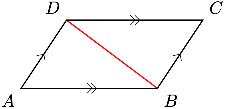
Problem 2. Show that the following are equivalent for a given quadrilateral :
is a parallelogram,
opposite sides in are equal,
opposite angles in are equal.
(Click for Solution)
Solution. Consider the parallelogram .
Draw the diagonal . Since , by alternate angles,
As a common side, . Since , by alternate angles,
By the ASA Criterion, . In particular, and , so that its opposite sides are equal.
Draw the diagonal and use the SSS Criterion to conclude that opposite angles equal each other.
Let denote the angles of the quadrilateral.
Since angles in a quadrilateral sum to ,
Since this equality holds for any pair of interior angles, the parallelogram must have two pairs of parallel sides.
Problem 3. Show that a rectangle is always a parallelogram. Furthermore, show that a parallelogram is a rectangle if and only if it has at least one interior right angle.
(Click for Solution)
Solution. Since all angles in a rectangle is , opposite pairs of angles are equal.
By Problem 2, a rectangle is a parallelogram.
Let denote the interior angles of the parallelogram, labelled anti-clockwise.
By Problem 2, and . Since angles in a quadrilateral sum to ,
Therefore, all angles equal , and the parallelogram is a rectangle.
Trivial.
Problem 4. Show that a rhombus is always a parallelogram. Furthermore, show that a parallelogram is a rhombus if and only if it has at least one pair of equal adjacent sides.
(Click for Solution)
Solution. Since opposite sides in a rhombus are equal, by Problem 2, a rhombus is a parallelogram.
Let denote the sides of a parallelogram, labelled anti-clockwise.
By Problem 2, and . By hypothesis, suppose without loss of generality. Then . Therefore, all side lengths are equal, and the parallelogram is a rhombus.
Trivial.
Problem 5. Show that a rectangle is a square if and only if it has at least one pair of equal adjacent sides. Likewise, show that a rhombus is a square if and only if it has at least one interior right angle.
(Click for Solution)
Solution. We first prove the rectangle claim:
By Problem 3, a rectangle is a parallelogram. By hypothesis and Problem 4, it is a rhombus. By Problem 1, it is a square.
Trivial.
The rhombus claim follows similarly:
By Problem 4, a rhombus is a parallelogram. By hypothesis and Problem 2, it is a rectangle. By Problem 1, it is a square.
Trivial.
Definition 4. A trapezium is a quadrilateral with at least one pair of opposite sides that are parallel.
Problem 6. Show that a parallelogram is always a trapezium. Furthermore, show that a trapezium is a parallelogram if and only if it has at least one pair of equal opposite angles.
(Click for Solution)
Solution. Since a parallelogram has two pairs of equal and parallel sides, it has at least one pair of parallel sides, and is thus a trapezium.
Denote the angles of the trapezium by .
Given the pair of parallel sides, interior angles are supplementary, so that
By Problem 2, the trapezium is a parallelogram.
Trivial.
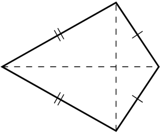
Definition 5. A kite is a quadrilateral with two pairs of adjacent sides that are equal in length.
Problem 7. Show that a kite has at least one pair of equal opposite angles and that its diagonals are perpendicular to each other.
(Click for Solution)
Solution. Consider the kite below.
As base angles of isosceles triangles,
Hence,
as required. Using the SAS Criterion, . In particular, . As a kite, . As base angles of an isosceles triangle,
Using the ASA Criterion, , so that . Since adjacent angles on a straight line are supplementary, . Solving, .
Problem 8. Show that a quadrilateral is a rhombus if and only if it is both a kite and a trapezium.
(Click for Solution)
Solution. Suppose the quadrilateral is both a kite and a trapezium. By Problem 7, it has at least one pair of equal opposite angles. By Problem 6, it is a parallelogram. As a kite, it has at least one pair of equal adjacent sides. By Problem 4, it is a rhombus.
If you won’t further your studies into a STEM discipline, then the tools and techniques in this post would not be terribly relevant for you. But for the aspiring STEM student, we are now going to do calculus with trigonometric functions and exponential functions.
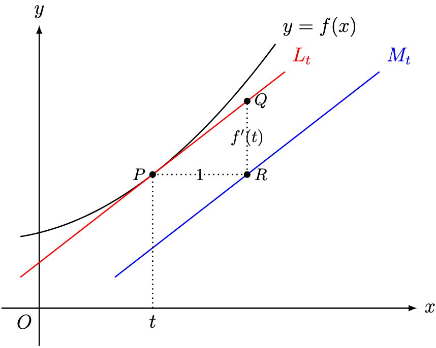
The derivative of is an exceedingly challenging idea to compute without more technical tool of limits outside the high school syllabus. To conceive of a meaningful derivation sacrifices either rigour or intuitiveness. Nevertheless, for this post, I will present the intuitive idea that appeared to me as I lay in my bed, fast asleep.
Denote . Derivatives intuitively measures the gradient of the tangent to the curve. Therefore, in the diagram below, I have computed the gradient of the tangent to each point on the curve . I colour-coded each point using the gradient at that point on a scale from very-red (i.e. gradient of ) to very-green (i.e. gradient of ). Hence, the graph goes from green to red, then back to green at the very end.
If now we plot the points of the new graph according to the colour-coding, the first quarter of the new graph lies in the top-half green section. The second and third quarters of the new graph lie in the bottom-half red section. And finally, the fourth quarter of the new graph lie in the top half-green section once again.
Recalling our discussions on trigonometric graphs, looks very much like the graph of . This is, in fact, mathematically true.
Theorem 1..
Proof. Omitted. Or relegated to a study in more advanced calculus. In the language of limits, we need to use the limit definition of the derivative to show that
Then the core result is proven using the limit
Remark 1. Strictly speaking, we have put the cart before the horse—I couldn’t colour the sine graph unless I already knew that the derivative of is . Nevertheless, the goal of this post is to motivate the result, then relegating a formal proof elsewhere in the blog.
You might wonder—in that case, why not obtain all other derivatives in this manner? Other than the fact that I need to slave-drive ChatGPT harder than I already do, it turns out that the existing differentiation technology, if we accept them to remain true for non-polynomials, empowers us to obtain (almost) all of these other derivatives.
For instance, the chain rule helps us compute the derivative of , since the complementary angle identities tell us that
Example 1. Show that .
Solution. Using the complementary angle identities, the chain rule, and Theorem 1,
These two results, coupled with the quotient rule, help us compute the derivative of , since . These reasons and more motivated our study on trigonometric identities.
Example 2. Show that .
Solution. Using the quotient rule and previous theorems,
There are many more commonly-used derivatives in this exercise here. We now state the integral versions of these three results.
Theorem 4. The following integrals hold:
Proof. We prove the first result to illustrate the power of thinking of integration as reverse differentiation. Using Theorem 2 and linearity,
Therefore dividing by on both sides,
where .
We have to discuss the exponential family too. Once again, just like with the derivative of , the derivative of requires more technical real-analytic tools to properly establish. Nevertheless, here is an experimentally-inspired attempt at motivating the result.
Let’s first ask ourselves: how can we experimentally compute the gradient of the tangent at a point on the graph of ? By definition, this tangent must pass through the point .
Draw a line parallel to the tangent passing through . We leave it as an exercise to check that its -intercept is given by the expression
In particular, if we know that has an -intercept of , then we can compute via
Now particularise to , which we can draw by sampling input values:
Notice that the -intercept of is exactly . This result is not a bug—it’s a feature of the graph of , and it works for any . In particular, using our “experimental” calculation of , we get
This result is a consequence of the famous differentiation result for exponentials.
Theorem 2..
Proof. Omitted.
Remark 2. Once again, we have assumed Theorem 2 in our illustration. A complete proof requires a rigorous definition of the real exponential, then deducing its various properties, and concluding by using the limit definition of the derivative. In the language of limits, the heart of the proof is the limit result
Recall that has a foil: the logarithm. More precisely, whenever well-defined,
Example 3. Show that for . The domain restriction allows the expression to make sense.
Solution. Using the chain rule and Theorem 2,
Remark 1. For , we have , so the chain rule yields
Therefore, the integral version of these results are given by
Since the absolute value is defined by
we can abbreviate the integral result as follows:
In particular, the absolute value symbol is essential in our final answer.
Definition 1. Define for by
Similarly, define for by
Likewise, define for real by
In particular,
The domain restrictions allow the expressions , , to make sense, similar to how the domain restriction allows the expression to make sense.
Example 4. Show that .
Solution. For the first result, use the chain rule and Theorem 1:
Since , , so that .
By the Pythagorean identity,
Therefore,
By definition,
Example 5. Show that .
Solution. Follow the strategy in Example 4 by using the chain rule and Example 2:
Using the Pythagorean identity,
Therefore,
By definition,
We conclude with one rather peculiar result regarding .
Example 6. Given that , show that
Solution. By the complementary angle identities,
Differentiating on both sides,
We have barely scratched the surface of calculus. There is much more that can be explored in many depths. At a high level, the area interpretation of integration allows mathematicians and statisticians to model probabilities—our conceived notions of randomness. We explore a special sub-branch of this topic next time.
What was the point of integration? To compute areas. Which sounds strange. Don’t we already have meaningful formulas for common areas?
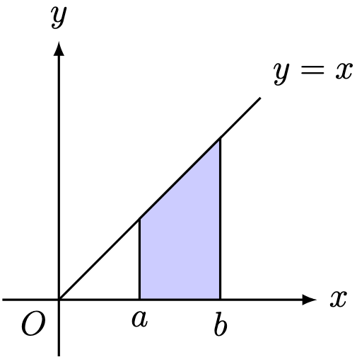
Example 1. Consider the graph below, with .
Define . Show that the shaded region has area
Solution. Using integration,
In particular,
Since the shaded region is a trapezium, it has an area given by
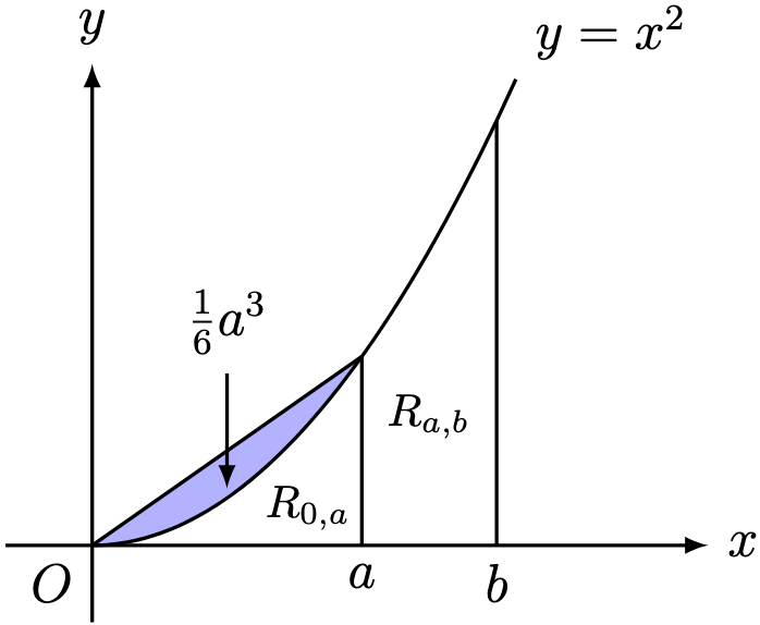
Example 2. Consider the graph below, with .
Define . The Greek mathematician Archimedes calculated the blue region to have an area of . Show that the area of is given by
Deduce that the area of is given by .
Solution. Using integration,
In particular, .
On the other hand, has area
The region can be thought of as the “leftover” region of after removing , and hence has area
This pattern turns out to be true in more general settings. We will simply state this general pattern, and omit its proof (referencing it for more a more advanced study of calculus).
Theorem 1. Consider the graph below, and suppose it lies above the -axis.
Define . Then the area of the shaded region is given by
Proof. This result is known as the famous fundamental theorem of calculus, which is rigorously proven elsewhere in the blog.
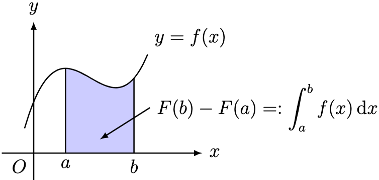
Definition 1. Given any function , make the notation
Suppose we know the functions such that
Then we define the definite integral of from to by
In particular, if lies above the -axis, then
denotes the area of the region in Theorem 1.
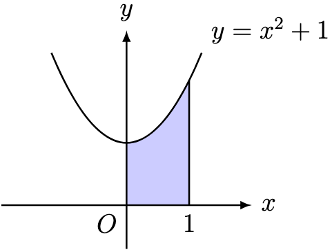
Example 3. For , evaluate .
Solution. Using integration,
Hence,
More generally, for any real ,
Using the definition of the definite integral, we can recover several important integration properties.
Theorem 2. Let be real constants with . Whenever well-defined, the following definite integral properties hold:
Proof. We will prove just the third result and relegate the rest of the results as exercises. Suppose satisfies
Then
Example 4. Evaluate the exact area of the following region.
Solution. Since the area under the graph is calculated using an integral,
Remark 1. Paradoxically, a rigorous treatment of calculus first proves Theorem 2 using a more fundamental definition of integration, then uses Theorem 2 and other real-analytic tools to prove Theorem 1.
Remark 2. The theory of integration is an incredibly deep rabbit hole, arguably deeper than that of differentiation. Its uses are deep and far-reaching due to its connections with probability (which influences basically almost every area of life). However, to keep things simple, we will restrict our attention to simple computations of integrals.
The rest of this post could evolve into a mere hodge-podge of integration drills, but perhaps we can think about Theorem 1 a little more closely.
Example 5. Consider the graph of below.
Evaluate and .
Solution. Using the linearity of integration
By Theorem 2,
If, instead, we graphed , the corresponding shaded region would lie below the -axis.
Furthermore, it would have an area of units².
Hence, strictly speaking, the integral only accounts for the signed area, which is positive if lies above the -axis, and negative if lies below the -axis.
In many ways, integration was formulated to answer problems in physics.
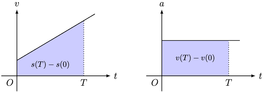
Definition 2. Sir Isaac Newton used calculus to formulate the connections between displacement, velocity, and acceleration at time as follows:
We remark that these definitions agree with the usual velocity-time graph (for displacement) and the acceleration-time graph (for velocity), where we calculate the desired quantities by evaluating the areas under the graphs (hence, corresponding with the integral formulation)
He was interested in the special case when is a constant number, namely , known as the gravitational acceleration near the surface of Earth.
Theorem 3. Given constants , suppose
.
Then
Furthermore, .
Proof. Integrating ,
Therefore,
Similarly,
where . Therefore,
In particular,
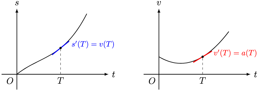
Theorem 3 lists out several common laws of kinematics, in particular, for an object moving in a straight line at constant acceleration. If instead we started by knowing the displacement , we can recover the velocity and acceleration of the particle using differentiation.
Theorem 4. The displacement , velocity , and acceleration of a particle moving in a straight line are related by the equations:
In particular, . This connection arises ubiquitously in physics due to Newton’s second law.
Proof. Write so that and
Differentiating on both sides,
The argument holds similarly for .
Similarly, these connections agree with the usual displacement-time graph (for velocity) and the velocity-time graph (for acceleration), where we calculate the desired quantities at a specific time by evaluating the gradient of the tangent at that point.
We have only scratched the surface regarding applied calculus, and you can explore even more in adjacent STEM fields like physics and economics.
For now, we need to answer a crucial question. So far, we have only discussed calculus regarding the simple-enough polynomials. But can we discuss calculus on the trigonometric functions like and , and the exponential family and of functions?
The answer is yes, sort of. A rigorous treatment takes a lot more effort into the nuts and bolts of calculus. Nevertheless, we can still appreciate these formulas from a visually intuitive perspective, and I think there is still a lot to enjoy from viewing it that way.
Remark 1. In both problems, we used the method of differences or a telescoping sum (or more fancifully, the fundamental theorem of discrete calculus), which states that if , then
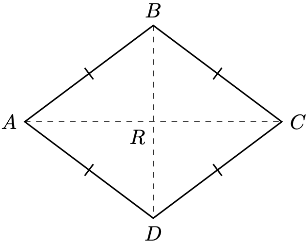
Definition 1. A rhombus is a shape made up of four straight line segments whose side lengths are all equal.
In the rhombus ABCD above, we call AC and BD the diagonals of the rhombus that intersect at R.
Problem 1. Show that the diagonals of a rhombus are perpendicular bisectors of each other.
(Click for Solution)
Solution. Since angles in a triangle are supplementary,
Since
summing the equations yields
Since , is isosceles, so that . Similarly,
Therefore,
Similarly, . Hence,
Since the interior angles sum to , . By alternate angles,
Using previous data, we have ,
By the ASA Criterion, . Similarly,
Therefore, and . Furthermore, since adjacent angles on a straight line are supplementary,
so that , and similarly,
Therefore, and are perpendicular bisectors of each other.
Problem 2. Let AB be the line segment below, and let r > 0 be a length such that
AB/2 < r ≤ AB.
Here, CA is a circle with centre A and radius r. Define CB likewise. Let P, Q denote the intersections between CA, CB.
Show that the line passing through P, Q is the perpendicular bisector of AB.
(Click for Solution)
Solution. As radii of the same circle,
Therefore, forms a rhombus. By Problem 1, lies on the perpendicular bisector of .
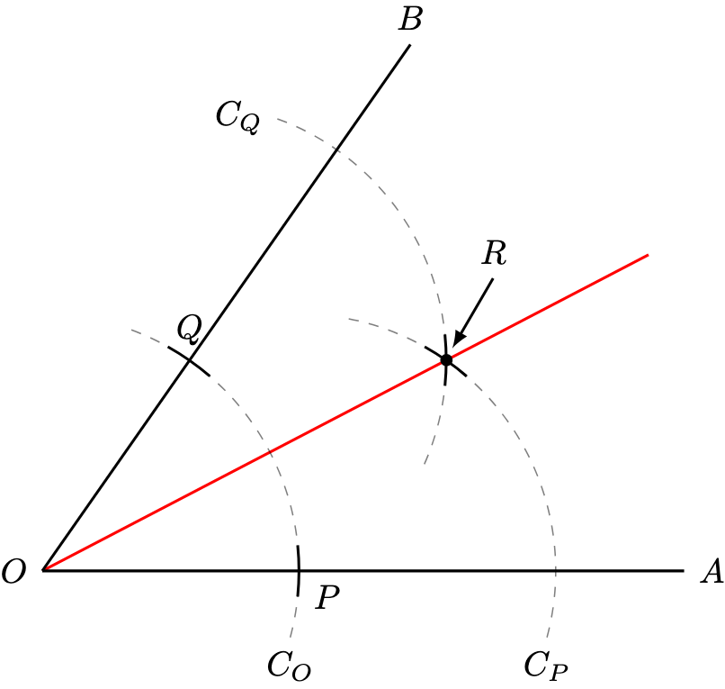
Problem 3. Let OA, OB be the line segments below, and let r > 0 be any length.
Here, CO denotes the circle with centre O and radius r. Suppose CO intersects OA at P and OB at Q. Define CA, CB similarly, and denote their intersection by R.
Show that ∠AOR = ∠BOR. In this case, we call the line passing through O, R the angle bisector of ∠AOB.
(Click for Solution)
Solution. As radii of the same circle,
Therefore, forms a rhombus. By Problem 1, and are perpendicular bisectors of each other.
Denote their intersection by . Then , , and . By the SSS Criterion, . In particular,
Let’s introduce baby integration as reverse-differentiation, which, comically, I have criticised elsewhere on my blog.
Given functions and , write
We call the left-hand equation the indefinite integral of with respect to.
(Wrong) Example 1. Recall that . Therefore,
Now strictly speaking, our integrals are wrong.
Lemma 1. Suppose and are functions such that
Then, for any real number ,
Proof. Using the linearity of differentiation,
Therefore, we use the following definition for indefinite integrals.
Definition 1. Given functions and , write
where is an arbitrary constant of integration.
Example 1. Recall that . Therefore, for ,
Now, Definition 1 is far from complete, but works well enough for most secondary-school assessments.
Theorem 1. Indefinite integration is linear: given functions and any real constant ,
Proof. Write
so that
By the linearity of differentiation,
For the second result, the linearity of differentiation yields
By Definition 1,
Example 2. For any , evaluate . In particular, for any constant , evaluate
Solution. From Example 1, if , then
Hence, writing , for ,
By the linearity of integration,
Therefore,
Since is still an arbitrary real constant,
The other results follow from linearity and the law of exponents:
Example 3. Evaluate .
Solution. Expanding yields
Since integration is linear,
Remark 1. Where possible, it is good practice to present your final answer as a sum of terms of the form , where are constants with being a positive integer and is not a polynomial.
Example 3 should suggest that computing integrals exactly would require a lot more effort than computing derivatives exactly. That is correct. For instance, we don’t actually yet know how to calculate
since Example 2 only works for .
Eventually, we will see that
which should surprise us—how did the logarithm magically appear there? For another fun result,
What else could we do with integration?
Example 4. Let be real constants. Evaluate . Hence, evaluate
Solution. Using the chain rule,
By Definition 1 and the linearity of integration,
where is an arbitrary real constant of integration.
Using the same idea in Example 4, we have the following special form of integration.
Theorem 2. If , then for real constants ,
Proof. Using the chain rule,
By Definition 1 and the linearity of integration,
where is an arbitrary real constant of integration.
Remark 1.Theorem 2 is a very special case of integrating by substitution, which is, in spirit, simply the reverse of the usual chain rule in differentiation.
Example 5. Differentiate . Hence, using Example 3, evaluate
Solution. Using the product rule and the chain rule,
Integrating on both sides and using linearity,
Doing algebra and using Example 3,
where is an arbitrary real constant of integration.
Remark 2.Example 5 is a guided example of integrating by parts, which is, in spirit, simply the reverse of the usual product rule in differentiation.
There is a lot more to say about integration, especially since we have not even discussed calculus involving the non-algebraic functions like the trigonometric functions , , , as well as the exponential function and its inverse the natural logarithm .
Nevertheless, we will push these discussions to the final post on integration, and pursue the essentials of the topic first. These functions have massive uses in the STEM fields, but for now we want to cover the big-idea bases of calculus that do not necessarily require them.
As such, we will apply integration to computing areas, as well as discuss some basic physics.
Theorem 1 (Product Rule). For functions with derivatives ,
Proof. We have the result
On the other hand, using vanilla algebra,
Hence,
Using linearity,
Previously, we have also proven that
Together with the product rule, we can prove the quotient rule.
Theorem 2 (Quotient Rule). For ,
Proof. Using the product rule,
Most differentiation problems becomes simply applying these results one after another, ensuring very careful algebraic calculations.
Example 1. Given that , , and , show that
Solution. Using the quotient rule,
Since ,
Since ,
The equation is called the zero derivative condition, which plays a vital role in optimisation applications.
Oddly enough, when compared with the chain rule, there is really not much else to be discussed about these two rules until we start differentiating other kinds of functions, like the trigonometric functions, exponential functions, and logarithm functions.
So for now, we switch gears and discuss turning points, applying it in the context of optimisation.


![\begin{aligned} z^3 &= m \pm \sqrt{m^2 - p} \\ z^3 &= -\frac D2 \pm \sqrt{\frac{D^2}{4} + \frac{C^3}{27}} \\ z_{\pm} &:= \sqrt[3]{ -\frac D2 \pm \sqrt{\frac{D^2}{4} + \frac{C^3}{27}} }. \end{aligned}](https://s0.wp.com/latex.php?latex=%5Cbegin%7Baligned%7D+z%5E3+%26%3D+m+%5Cpm+%5Csqrt%7Bm%5E2+-+p%7D+%5C%5C+z%5E3+%26%3D+-%5Cfrac+D2+%5Cpm+%5Csqrt%7B%5Cfrac%7BD%5E2%7D%7B4%7D+%2B+%5Cfrac%7BC%5E3%7D%7B27%7D%7D+%5C%5C+z_%7B%5Cpm%7D+%26%3A%3D+%5Csqrt%5B3%5D%7B+-%5Cfrac+D2+%5Cpm+%5Csqrt%7B%5Cfrac%7BD%5E2%7D%7B4%7D+%2B+%5Cfrac%7BC%5E3%7D%7B27%7D%7D+%7D.+%5Cend%7Baligned%7D&bg=ffffff&fg=000&s=0&c=20201002)


 .
.


 .
. . In particular,


 . By Problem 1,


 to
to  .
.

 comes from Problem 2. Multiplying both sides by
  yields the formula
 -gon with vertices

 .
.
 Suppose a quadrilateral is both a rectangle and a rhombus.
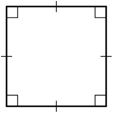
 Trivial.
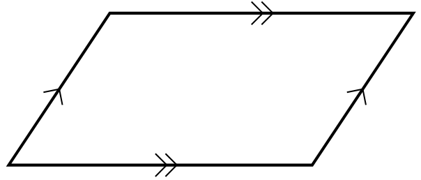
 :
: Consider the parallelogram
  .
.
 . Since
  , by alternate angles,
 . Since
  , by alternate angles,
 . In particular,
  and
and  , so that its opposite sides are equal.
 Draw the diagonal and use the SSS Criterion to conclude that opposite angles equal each other.
 Let
Let  denote the angles of the quadrilateral.
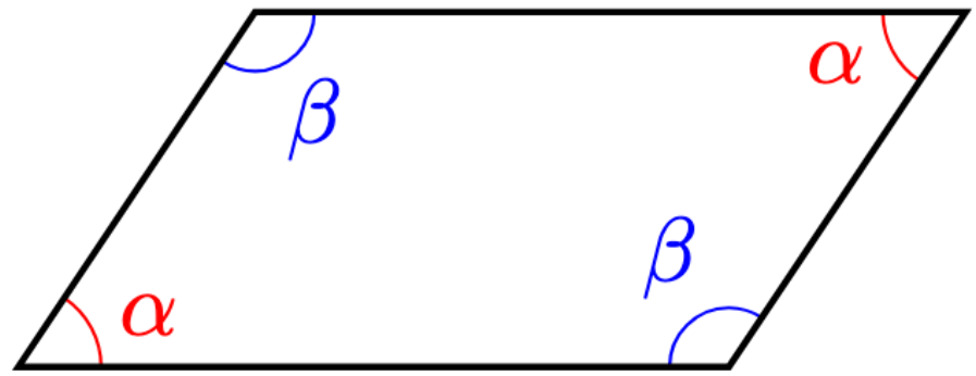
 ,
,
 denote the interior angles of the parallelogram, labelled anti-clockwise.
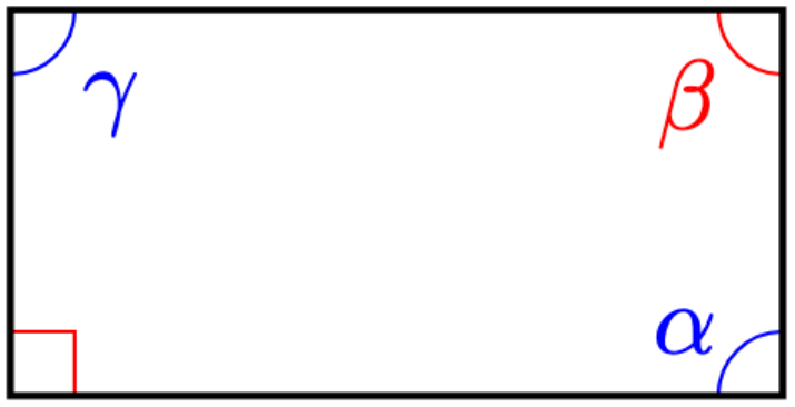
 and
and  . Since angles in a quadrilateral sum to
 denote the sides of a parallelogram, labelled anti-clockwise.
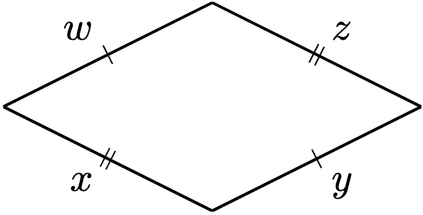
 and
and  . By hypothesis, suppose
  without loss of generality. Then
  . Therefore, all side lengths are equal, and the parallelogram is a rhombus.
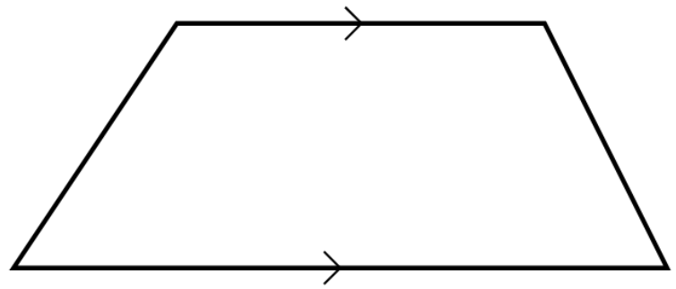
 .
.

 below.
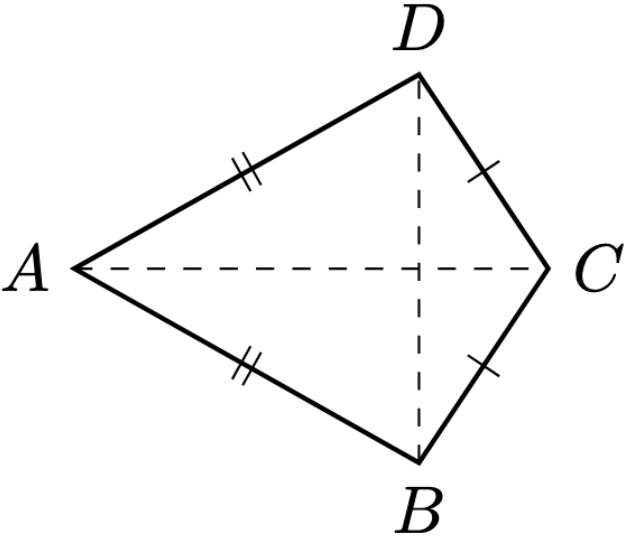


 . In particular,
  . As a kite,
  . As base angles of an isosceles triangle,
 , so that
  . Since adjacent angles on a straight line are supplementary,
  . Solving,
  .
.

 with
with  ,
,

 be integers.
 and
and  . Show that the quadratic equation
 .
. . Using the quadratic formula, the solutions are given by

 , evaluate
  in terms of
  . Deduce that
 .
.
 and by Problem 1,
 and
and  . Hence,
 .
. is a positive integer.
 . Evaluate
 .
.
 , by calculating the discriminant of the quadratic equation,
 such that
 :
:
 .
. , show that

 . Dividing by
  yields the desired result.
 is an exceedingly challenging idea to compute without more technical tool of limits outside the high school syllabus. To conceive of a meaningful derivation sacrifices either rigour or intuitiveness. Nevertheless, for this post, I will present the intuitive idea that appeared to me as I lay in my bed, fast asleep.
 . Derivatives intuitively measures the gradient of the tangent to the curve. Therefore, in the diagram below, I have computed the gradient of the tangent to each point on the curve
  . I colour-coded each point
  using the gradient
  at that point on a scale from very-red (i.e. gradient of
  ) to very-green (i.e. gradient of
  ). Hence, the graph goes from green to red, then back to green at the very end.
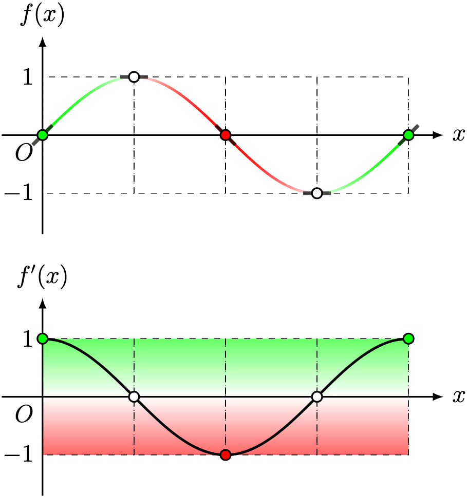
 according to the colour-coding, the first quarter of the new graph lies in the top-half green section. The second and third quarters of the new graph lie in the bottom-half red section. And finally, the fourth quarter of the new graph lie in the top half-green section once again.
 looks very much like the graph of
  . This is, in fact, mathematically true.
 .
.

 is
is  . Nevertheless, the goal of this post is to motivate the result, then relegating a formal proof elsewhere in the blog.
 .
.
 , since
  . These reasons and more motivated our study on
  .
.


 .
. requires more technical
  at a point
  on the graph of
  .
.
 parallel to the tangent passing through
  . We leave it as an exercise to check that its
  -intercept
  is given by the expression

 , which we can draw by sampling input values:
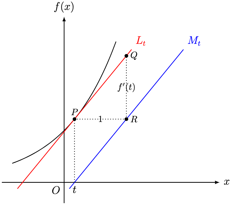
 . This result is not a bug—it’s a feature of the graph of
  , and it works for any
  . In particular, using our “experimental” calculation of
 .
.

 for
for  . The domain restriction
  to make sense.
 , we have
  , so the chain rule yields


 is essential in our final answer.
 for
for  by
by
 for
for 
 for real

 ,
,  ,
,  to make sense, similar to how the domain restriction
  .
.
 ,
,  , so that
  .
.


 .
.


 below, with
  .
.
 . Show that the shaded region has area


 below, with
  .
.
 . The Greek mathematician Archimedes calculated the blue region to have an area of
  . Show that the area of
  is given by
 is given by
  .
.
 .
.
 after removing
 . Then the area of the shaded region is given by
 , make the notation
![[G(x)]_a^b := G(b) - G(a).](https://s0.wp.com/latex.php?latex=%5BG%28x%29%5D_a%5Eb+%3A%3D+G%28b%29+-+G%28a%29.&bg=ffffff&fg=000&s=0&c=20201002)
 such that
 from
from  to
to ![\displaystyle \int_a^b f(x)\, \mathrm dx := [F(x)]_a^b \equiv F(b) - F(a).](https://s0.wp.com/latex.php?latex=%5Cdisplaystyle+%5Cint_a%5Eb+f%28x%29%5C%2C+%5Cmathrm+dx+%3A%3D+%5BF%28x%29%5D_a%5Eb+%5Cequiv+F%28b%29+-+F%28a%29.&bg=ffffff&fg=000&s=0&c=20201002)

 , evaluate
  .
.
![\displaystyle \int_0^1 x^n\, \mathrm dx = \left[ \frac{x^{n+1}}{n+1} \right]_0^1 = \frac{1^{n+1}}{n+1} - \frac{0^{n+1}}{n+1} = \frac 1{n+1}.](https://s0.wp.com/latex.php?latex=%5Cdisplaystyle+%5Cint_0%5E1+x%5En%5C%2C+%5Cmathrm+dx+%3D+%5Cleft%5B+%5Cfrac%7Bx%5E%7Bn%2B1%7D%7D%7Bn%2B1%7D+%5Cright%5D_0%5E1+%3D+%5Cfrac%7B1%5E%7Bn%2B1%7D%7D%7Bn%2B1%7D+-+%5Cfrac%7B0%5E%7Bn%2B1%7D%7D%7Bn%2B1%7D+%3D+%5Cfrac+1%7Bn%2B1%7D.&bg=ffffff&fg=000&s=0&c=20201002)

 be real constants with
  . Whenever well-defined, the following definite integral properties hold:
 satisfies
![\begin{aligned} \int_a^b f(x) \, \mathrm dx + \int_b^c f(x) \, \mathrm dx &= [F(x)]_a^b + [F(x)]_b^c \\ &= (F(b) - F(a)) + (F(c) - F(b)) \\ &= F(c) - F(a) \\ &= \int_a^c f(x) \, \mathrm dx. \end{aligned}](https://s0.wp.com/latex.php?latex=%5Cbegin%7Baligned%7D+%5Cint_a%5Eb+f%28x%29+%5C%2C+%5Cmathrm+dx+%2B+%5Cint_b%5Ec+f%28x%29+%5C%2C+%5Cmathrm+dx+%26%3D+%5BF%28x%29%5D_a%5Eb+%2B+%5BF%28x%29%5D_b%5Ec+%5C%5C+%26%3D+%28F%28b%29+-+F%28a%29%29+%2B+%28F%28c%29+-+F%28b%29%29+%5C%5C+%26%3D+F%28c%29+-+F%28a%29+%5C%5C+%26%3D+%5Cint_a%5Ec+f%28x%29+%5C%2C+%5Cmathrm+dx.++%5Cend%7Baligned%7D&bg=ffffff&fg=000&s=0&c=20201002)

 below.
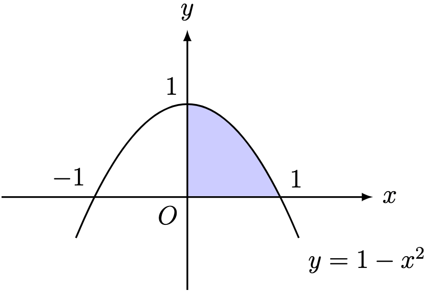
 and
and  .
.

 , the corresponding shaded region would lie below the
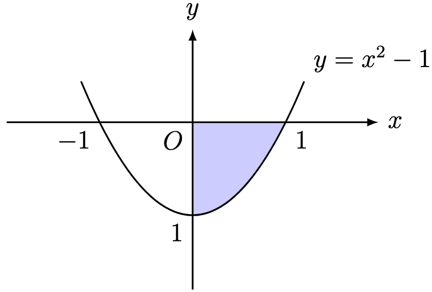
 units².
 , velocity
  , and acceleration
  at time
  as follows:
 is a constant number, namely
  , known as the gravitational acceleration near the surface of Earth.
 , suppose
 .
.
 .
.
![\begin{aligned} v(T) &= v(0) + \int_0^T a(t)\, \mathrm dt \\ &= v_0 + [a_0x]_0^T \\ &= v_0 + (a_0 T - a_0 \cdot 0) \\ &= v_0 + a_0T. \end{aligned}](https://s0.wp.com/latex.php?latex=%5Cbegin%7Baligned%7D+v%28T%29+%26%3D+v%280%29+%2B+%5Cint_0%5ET+a%28t%29%5C%2C+%5Cmathrm+dt+%5C%5C+%26%3D+v_0+%2B+%5Ba_0x%5D_0%5ET+%5C%5C+%26%3D+v_0+%2B+%28a_0+T+-+a_0+%5Ccdot+0%29+%5C%5C+%26%3D+v_0+%2B+a_0T.+%5Cend%7Baligned%7D&bg=ffffff&fg=000&s=0&c=20201002)

 . Therefore,
![\begin{aligned} s(T) &= s(0) + \int_0^T v(t)\, \mathrm dt \\ &= \textstyle s_0 + \left[ v_0t + \frac 12 a_0t^2 \right]_0^T \\ &= \textstyle s_0 + \left( v_0T + \frac 12 a_0T^2 \right) - \left( v_0\cdot 0 + \frac 12 a_0 \cdot 0^2 \right) \\ &= \textstyle s_0 + v_0T + \frac 12 a_0T^2 . \end{aligned}](https://s0.wp.com/latex.php?latex=%5Cbegin%7Baligned%7D+s%28T%29+%26%3D+s%280%29+%2B+%5Cint_0%5ET+v%28t%29%5C%2C+%5Cmathrm+dt+%5C%5C+%26%3D+%5Ctextstyle+s_0+%2B+%5Cleft%5B+v_0t+%2B+%5Cfrac+12+a_0t%5E2+%5Cright%5D_0%5ET+%5C%5C+%26%3D+%5Ctextstyle+s_0+%2B+%5Cleft%28+v_0T+%2B+%5Cfrac+12+a_0T%5E2+%5Cright%29+-+%5Cleft%28+v_0%5Ccdot+0+%2B+%5Cfrac+12+a_0+%5Ccdot+0%5E2+%5Cright%29+%5C%5C+%26%3D+%5Ctextstyle+s_0+%2B+v_0T+%2B+%5Cfrac+12+a_0T%5E2+.+%5Cend%7Baligned%7D&bg=ffffff&fg=000&s=0&c=20201002)

 , we can recover the velocity and acceleration of the particle using differentiation.
 , and acceleration
 . This connection arises ubiquitously in physics due to Newton’s second law.
 so that
  and
and


 ,
,

 , then


 ,
,  is isosceles, so that
  . Similarly,

 . Hence,
 ,
, 
 ,
,
 . Similarly,
 and
and  . Furthermore, since adjacent angles on a straight line are supplementary,

 and
and 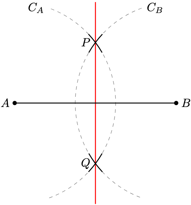

 forms a rhombus. By Problem 1,
  lies on the perpendicular bisector of
  .
.

 forms a rhombus. By Problem 1,
  are perpendicular bisectors of each other.
 . Then
  ,
,  , and
, and  . By the SSS Criterion,
  . In particular,

 . Therefore,

 ,
,


 ,
,
 and any real constant


 . In particular, for any constant
 , then
 , for
, for 


 is still an arbitrary real constant,

 .
. yields

 , where
  are constants with


 . Hence, evaluate


 is an arbitrary real constant of integration.
 , then for real constants


 is an arbitrary real constant of integration.
 . Hence, using Example 3, evaluate


 is an arbitrary real constant of integration.
 and
and  , we have

 ,
,


 ,
,

 ,
,  , show that


 is called the zero derivative condition, which plays a vital role in optimisation applications.