Milk Tea Matrices

Let’s drink some milk tea! Consider the three milk tea chains in Singapore: Chagee, Koi, and LiHo. (There are many others, so please experiment with these other chains if you wish.)

Let $c_t, k_t, \ell_t$ denote the proportion of the population that drinks Chagee, Koi, and LiHo respectively at time $t$ , measured in months. For simplicity, assume that customers are exclusive and loyal—Chagee drinkers do not drink from Koi and vice versa.

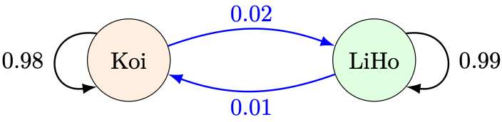
Before Chagee came on the scene, the milk tea scene was mostly split between Koi and LiHo, so that $c_0 = 0$ . Let’s suppose that 50% of the population drank Koi and 50% of the population drank LiHo at time t, measured in months, so that $k_0 = 0.5$ and $\ell_0 = 0.5$ . Since LiHo is newer than Koi, suppose the following changes happen after each month:

2% of Koi drinkers switch to LiHo,
1% of LiHo drinkers switch to Koi.

Example 1. At the end of the first month, what proportion of the population would be Koi drinkers?

Solution. We can represent these changes using the following diagram. Arrows once again represent similar ideas as they do in probability tree diagrams: the arrow from Koi to LiHo with label 0.02 means that 0.02 of Koi drinkers switch to LiHo.

Recall that $c_1, k_1, \ell_1$ denotes the proportion of the population that drinks Chagee, Koi, and LiHo respectively at the end of month $1$ . Since Chagee has not yet existed in the Singapore market, $c_1 = 0$ . Now $k_1$ is determined by two quantities:

the 98% of Koi customers who remained loyal to Koi,
the 1% of LiHo customers who switched to Koi.

Therefore,

$k_1 = 0.98 \cdot k_0 + 0.01 \cdot \ell_0.$

Similarly,

$\ell_1 = 0.02\cdot k_0 + 0.99\cdot \ell_0.$

Since $k_0 = \ell_0 = 0.5$ , we can substitute them into both equations and obtain $k_1$ as our desired answer:

$\begin{aligned} k_1 &= 0.98 \cdot 0.5 + 0.01 \cdot 0.5 = 0.495, \\ \ell_1 &= 0.02 \cdot 0.5 + 0.99 \cdot 0.5 = 0.505.\end{aligned}$

Indeed, Koi lost a small amount of its market share, as predicted.

Now suppose the proportion of drinkers as per Example 1. For reasons that will become apparent later, let’s denote the market shares as vectors:

$\mathbf x_t = \begin{bmatrix} c_t \\ k_t \\ \ell_t \end{bmatrix}\quad \Rightarrow \quad \mathbf x_1 = \begin{bmatrix} c_1 \\ k_1 \\ \ell_1 \end{bmatrix} = \begin{bmatrix} 0 \\ 0.495 \\ 0.505 \end{bmatrix}.$

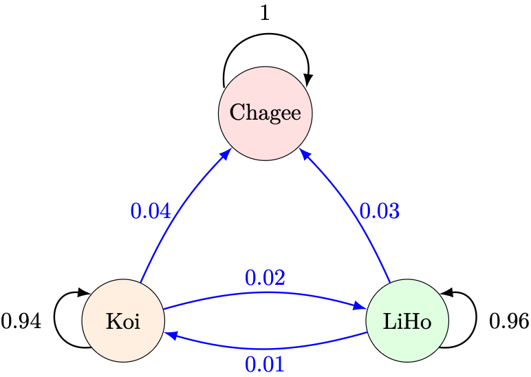
Due to aggressive social media marketing by Chagee’s youthful team, suppose at the end of every month, the following changes happen after each month:

4% of Koi drinkers switch to Chagee,
3% of LiHo drinkers switch to Chagee.
All Chagee drinkers keep drinking Chagee.

Question 1. At the end of the second month, what proportion of the population would be Chagee drinkers?

We can represent these changes using the following diagram, now including Chagee in our calculations.

Using similar analysis to Example 1, we write out the following three equations:

$\begin{aligned} c_2 &= 1 \cdot c_1 + 0.04 \cdot k_1 + 0.03 \cdot \ell_1, \\ k_2 &= 0 \cdot c_1 + 0.94 \cdot k_1 + 0.01 \cdot \ell_1, \\ \ell_2 &= 0 \cdot c_1 + 0.02 \cdot k_2 + 0.96 \cdot \ell_2.\end{aligned}$

Use vector notation to simplify our work:

$\begin{aligned} \begin{bmatrix} c_2 \\ k_2 \\ \ell_2 \end{bmatrix} &= \begin{bmatrix} 1 \cdot c_1 + 0.04 \cdot k_1 + 0.03 \cdot \ell_1 \\ 0 \cdot c_1 + 0.94 \cdot k_1 + 0.01 \cdot \ell_1 \\ 0 \cdot c_1 + 0.02 \cdot k_2 + 0.96 \cdot \ell_2 \end{bmatrix} \\ &= \begin{bmatrix} 1 \cdot c_1 \\ 0 \cdot c_1 \\ 0 \cdot c_1 \end{bmatrix} + \begin{bmatrix} 0.04 \cdot k_1 \\ 0.94 \cdot k_1 \\ 0.02 \cdot k_2 \end{bmatrix} + \begin{bmatrix} 0.03 \cdot \ell_1 \\ 0.01 \cdot \ell_1 \\ 0.96 \cdot \ell_2 \end{bmatrix} \\ &= c_1 \begin{bmatrix} 1 \\ 0 \\ 0 \end{bmatrix} + k_1 \begin{bmatrix} 0.04 \\ 0.94 \\ 0.02 \end{bmatrix} + \ell_1 \begin{bmatrix} 0.03 \\ 0.01 \\ 0.96 \end{bmatrix}\end{aligned}$

At this point in time, all we need to do is to substitute $c_1 = 0$ , $k_1 = 0.495$ , and $\ell_1 = 0.505$ to obtain our answer (as an exercise, check that $c_2 = 0.03495$ ). But what if we wanted to re-use this information to answer more sophisticated questions? Wouldn’t it be nice to condense this information even further?

Remark 1. The setups we gave are specific kinds of Markov chains and more generally, stochastic processes, an model of describing sequences of random variables that satisfy sufficiently nice probability properties.

We can think of the three vectors as the “ingredients” needed that produce our result, while the numbers $c_1, k_1, \ell_1$ denote a “recipe” in combining these ingredients. To that end, mathematicians and statisticians stack the ingredients side-by-side as a matrix, and place the “recipe” vector on the right-hand side:

$\displaystyle c_1 \begin{bmatrix} 1 \\ 0 \\ 0 \end{bmatrix} + k_1 \begin{bmatrix} 0.04 \\ 0.94 \\ 0.02 \end{bmatrix} + \ell_1 \begin{bmatrix} 0.03 \\ 0.01 \\ 0.96 \end{bmatrix} = \begin{bmatrix} 1 & 0.04 & 0.03 \\ 0 & 0.94 & 0.01 \\ 0 & 0.02 & 0.96 \end{bmatrix} \begin{bmatrix} c_1 \\ k_1 \\ \ell_1 \end{bmatrix}.$

This is, in fact, the essential origin-story of the matrix. It wasn’t a-priori defined as a table of numbers equipped with some out-of-the-blue calculations; it was simply a summary of changing data!

Remark 2. Notice that the notion of a 3-dimensional vector just arose from our problem setup. In the physical world, we can still visualise 3 dimensions, but more complicated setups would require the use of $n$ -dimensional vectors, where $n > 3$ . In these settings, physical intuition fails, but we can still reason about them through formalised mathematical definitions.

Definition 1. An $m \times 1$ matrix is an $m$ -dimensional vector. For example, we have the following $3 \times 1$ matrix $\mathbf x_1$ :

$\mathbf x_1 = \begin{bmatrix} c_1 \\ k_1 \\ \ell_1 \end{bmatrix} = \begin{bmatrix} 0 \\ 0.495 \\ 0.505\end{bmatrix}.$

An $m \times n$ matrix is a collection of $n$ vectors, each of them $m$ -dimensional, placed beside each other:

$\mathbf A = \begin{bmatrix} \mathbf a_1 & \cdots & \mathbf a_n \end{bmatrix}$

For example, we have the following $3 \times 3$ matrix $\mathbf A$ and $2 \times 3$ matrix $\mathbf B$ :

$\mathbf A = \begin{bmatrix} 1 & 0.04 & 0.03 \\ 0 & 0.94 & 0.01 \\ 0 & 0.02 & 0.96 \end{bmatrix}, \quad \mathbf B = \begin{bmatrix} 1 & 2 & 3 \\ 4 & 5 & 6 \end{bmatrix}.$

Furthermore, given an $n$ -dimensional vector $\mathbf v = \begin{bmatrix} v_1 \\ \vdots \\ v_n \end{bmatrix}$ , we define the expression $\mathbf A \mathbf v$ to mean

$\mathbf A \mathbf v \equiv \begin{bmatrix} \mathbf a_1 & \cdots & \mathbf a_n \end{bmatrix}\begin{bmatrix} v_1 \\ \vdots \\ v_n \end{bmatrix} := v_1 \mathbf a_1 + \cdots + v_n \mathbf a_n.$

Define the zero matrix by $\mathbf 0 := \begin{bmatrix} \mathbf 0 & \cdots & \mathbf 0 \end{bmatrix}$ .

Example 2. Evaluate the expression

$\begin{bmatrix} 1 & 2 & 3 \\ 4 & 5 & 6 \end{bmatrix} \begin{bmatrix} 7 \\ 8 \\ 9 \end{bmatrix},$

giving your answer in terms of a 2-dimensional vector.

Solution. Using Definition 1,

$\begin{aligned} \begin{bmatrix} 1 & 2 & 3 \\ 4 & 5 & 6 \end{bmatrix} \begin{bmatrix} 7 \\ 8 \\ 9 \end{bmatrix} &= 7 \begin{bmatrix} 1 \\ 4 \end{bmatrix} + 8 \begin{bmatrix} 2 \\ 5 \end{bmatrix} + 9 \begin{bmatrix} 3 \\ 6 \end{bmatrix} \\ &= \begin{bmatrix} 7 \\ 28 \end{bmatrix} + \begin{bmatrix} 16 \\ 40 \end{bmatrix} + \begin{bmatrix} 27 \\ 54 \end{bmatrix} \\ &= \begin{bmatrix} 7 + 16 + 27 \\ 28 + 40 + 54 \end{bmatrix} \\ &= \begin{bmatrix} 50 \\ 114 \end{bmatrix}. \end{aligned}$

Remark 2. The expression in Example 2, being contrived, doesn’t represent any particular real-world example. However, its calculations are identical to that of the milk tea example (which is, itself, not entirely faithful to reality, but simplified for analogous purposes).

Example 3. Given an $m \times n$ matrix $\mathbf A$ , how many dimensions must the vector $\mathbf v$ have so that $\mathbf A\mathbf v$ makes sense?

Solution. Write

$\mathbf A = \begin{bmatrix} \mathbf a_1 & \cdots & \mathbf a_n \end{bmatrix},$

where each $\mathbf a_1,\dots,\mathbf a_n$ is an $m$ -dimensional vector. Since $\mathbf A$ has $n$ “ingredients” that combined with “recipe” vector $\mathbf v$ gives the “dishes” $\mathbf A\mathbf v$ , our “recipe” vector $\mathbf v$ should have $n$ components. That is, $\mathbf v$ should be $n$ -dimensional.

If we could add vectors, could we add matrices? The real question is, why not? Consider the two expressions below:

$\begin{aligned} \begin{bmatrix} 1 & 2 & 3 \\ 4 & 5 & 6 \end{bmatrix} \begin{bmatrix} 7 \\ 8 \\ 9 \end{bmatrix},\quad \begin{bmatrix} 10 & 11 & 12 \\ 13 & 14 & 15 \end{bmatrix} \begin{bmatrix} 7 \\ 8 \\ 9 \end{bmatrix} \end{aligned}.$

Let’s expand both terms using the recipe-ingredient analogy:

$\begin{aligned} \begin{bmatrix} 1 & 2 & 3 \\ 4 & 5 & 6 \end{bmatrix} \begin{bmatrix} 7 \\ 8 \\ 9 \end{bmatrix} &= 7 \begin{bmatrix} 1 \\ 4 \end{bmatrix} + 8 \begin{bmatrix} 2 \\ 5 \end{bmatrix} + 9 \begin{bmatrix} 3 \\ 6 \end{bmatrix},\\ \begin{bmatrix} 10 & 11 & 12 \\ 13 & 14 & 15 \end{bmatrix} \begin{bmatrix} 7 \\ 8 \\ 9 \end{bmatrix} &= 7 \begin{bmatrix} 10 \\ 13 \end{bmatrix} + 8 \begin{bmatrix} 11 \\ 14 \end{bmatrix} + 9 \begin{bmatrix} 12 \\ 15 \end{bmatrix}. \end{aligned}$

Now let’s add both sides of the equation together:

$\begin{aligned} &\begin{bmatrix} 1 & 2 & 3 \\ 4 & 5 & 6 \end{bmatrix} \begin{bmatrix} 7 \\ 8 \\ 9 \end{bmatrix} + \begin{bmatrix} 10 & 11 & 12 \\ 13 & 14 & 15 \end{bmatrix} \begin{bmatrix} 7 \\ 8 \\ 9 \end{bmatrix} \\ &= 7 \left( \begin{bmatrix} 1 \\ 4 \end{bmatrix} + \begin{bmatrix} 10 \\ 13 \end{bmatrix} \right) + 8 \left(\begin{bmatrix} 2 \\ 5 \end{bmatrix} + \begin{bmatrix} 11 \\ 14 \end{bmatrix}\right) + 9 \left(\begin{bmatrix} 3 \\ 6 \end{bmatrix} + \begin{bmatrix} 12 \\ 15 \end{bmatrix}\right) \\ &= 7 \begin{bmatrix} 1 + 10 \\ 4 + 13 \end{bmatrix} + 8 \begin{bmatrix} 2 + 11 \\ 5 + 14 \end{bmatrix} + 9 \begin{bmatrix} 3 + 12 \\ 6 + 15 \end{bmatrix} \\ &= \begin{bmatrix} 1 + 10 & 2 + 11 & 3 + 12 \\ 4 + 13 & 5 + 14 & 6 + 15\end{bmatrix} \begin{bmatrix} 7 \\ 8 \\ 9 \end{bmatrix}, \end{aligned}$

where we consolidated our calculations using the recipe-ingredient analogy again. Therefore, it is reasonable to define

$\begin{bmatrix} 1 & 2 & 3 \\ 4 & 5 & 6 \end{bmatrix} + \begin{bmatrix} 10 & 11 & 12 \\ 13 & 14 & 15 \end{bmatrix} := \begin{bmatrix} 1 + 10 & 2 + 11 & 3 + 12 \\ 4 + 13 & 5 + 14 & 6 + 15\end{bmatrix},$

so that for any 3-dimensional vector $\mathbf u = \begin{bmatrix}u_1 \\ u_2 \\ u_3\end{bmatrix}$ ,

$\left( \begin{bmatrix} 1 & 2 & 3 \\ 4 & 5 & 6 \end{bmatrix} + \begin{bmatrix} 10 & 11 & 12 \\ 13 & 14 & 15 \end{bmatrix} \right)\mathbf u = \begin{bmatrix} 1 & 2 & 3 \\ 4 & 5 & 6 \end{bmatrix} \mathbf u + \begin{bmatrix} 10 & 11 & 12 \\ 13 & 14 & 15 \end{bmatrix} \mathbf u.$

A similar thought process works for multiplying a matrix by a number (i.e. scalar multiplication) and matrix subtraction.

Definition 2. Let $\mathbf A =\begin{bmatrix} \mathbf a_1 & \cdots & \mathbf a_n\end{bmatrix}$ and $\mathbf B =\begin{bmatrix} \mathbf b_1 & \cdots & \mathbf b_n\end{bmatrix}$ be $m \times n$ matrices. Define matrix addition “ingredient-wise” by

$\mathbf A + \mathbf B :=\begin{bmatrix} \mathbf a_1 + \mathbf b_1 & \cdots & \mathbf a_n + \mathbf b_n\end{bmatrix},$

so that for any $n$ -dimensional vector $\mathbf v$ , $(\mathbf A + \mathbf B) \mathbf v = \mathbf A \mathbf v + \mathbf B \mathbf v$ .

Similarly, given any real number $c$ , define scalar multiplication “ingredient-wise” by

$c\mathbf A :=\begin{bmatrix} c\mathbf a_1 & \cdots & c\mathbf a_n\end{bmatrix},$

so that for any $n$ -dimensional vector $\mathbf v$ , $(c\mathbf A) \mathbf v = \mathbf A(c\mathbf v) = c(\mathbf A \mathbf v)$ .

In particular, define $-\mathbf A := (-1)\mathbf A$ , and $\mathbf A - \mathbf B := \mathbf A + (-\mathbf B)$ .

Example 4. Show that $(\mathbf A -\mathbf B)\mathbf v = \mathbf A \mathbf v - \mathbf B \mathbf v$ .

Solution. By Definition 2 and its implications,

$\begin{aligned} (\mathbf A -\mathbf B)\mathbf v &= (\mathbf A + (-\mathbf B))\mathbf v \\ &= \mathbf A\mathbf v + (-\mathbf B)\mathbf v \\ &= \mathbf A\mathbf v + ((-1)\mathbf B)\mathbf v \\ &= \mathbf A\mathbf v + (-1)(\mathbf B \mathbf v) \\ &= \mathbf A \mathbf v - \mathbf B \mathbf v. \end{aligned}$

Example 5. Evaluate the following expressions:

$\begin{bmatrix} 1 & -2 \\ 3 & 4 \\ 5 & -6 \end{bmatrix} + \begin{bmatrix} -10 & 11 \\ 12 & 13 \\ -14 & -15 \end{bmatrix},\quad 7\begin{bmatrix} 1 & 2 & 3 \\ 4 & 5 & 6 \end{bmatrix},\quad \begin{bmatrix} 1 & -2 \\ 3 & 4 \\ 5 & -6 \end{bmatrix} - \begin{bmatrix} -10 & 11 \\ 12 & 13 \\ -14 & -15 \end{bmatrix}.$

Solution. Using Definition 2,

$\begin{aligned} \begin{bmatrix} 1 & -2 \\ 3 & 4 \\ 5 & -6 \end{bmatrix} + \begin{bmatrix} -10 & 11 \\ 12 & 13 \\ -14 & -15 \end{bmatrix} &= \begin{bmatrix} -9 & 9 \\ 15 & 17 \\ -9 & -21\end{bmatrix},\\ 7\begin{bmatrix} 1 & 2 & 3 \\ 4 & 5 & 6 \end{bmatrix} &= \begin{bmatrix} 7 & 14 & 21 \\ 28 & 35 & 42 \end{bmatrix},\\ \begin{bmatrix} 1 & -2 \\ 3 & 4 \\ 5 & -6 \end{bmatrix} - \begin{bmatrix} -10 & 11 \\ 12 & 13 \\ -14 & -15 \end{bmatrix} &= \begin{bmatrix} 11 & -13 \\ -9 & -9 \\ 19 & 9 \end{bmatrix}.\end{aligned}$

Theorem 1. Given $m\times n$ matrices $\mathbf A,\mathbf B,\mathbf C$ and scalars $c, d$ , the following matrix properties hold:

$\mathbf A + \mathbf B = \mathbf B + \mathbf A$ ,
$(\mathbf A + \mathbf B) + \mathbf C = \mathbf A + (\mathbf B + \mathbf C)$ ,
$\mathbf A + \mathbf 0 = \mathbf 0 + \mathbf A$ ,
$\mathbf A + (-\mathbf A) = (-\mathbf A) + \mathbf A = \mathbf 0$ ,
$c(d\mathbf A) = (cd)\mathbf A$ ,
$1 \mathbf A = \mathbf A$ ,
$c(\mathbf A +\mathbf B) = c\mathbf A + c\mathbf B$ ,
$(c + d)\mathbf A = c\mathbf A + d\mathbf A$ .

Proof. Left as a tedious (but ultimately meaningful) exercise.

How might we multiply two matrices together? Consider the expression

$\mathbf A \begin{bmatrix} \mathbf v_1 & \mathbf v_2 \end{bmatrix}.$

Using the ingredient-recipe analogy, the matrix on the right-hand side has two recipes, not one. Therefore, we can think of the expression as cooking two dishes; this is our definition of matrix multiplication:

$\mathbf A \begin{bmatrix} \mathbf v_1 & \mathbf v_2 \end{bmatrix} := \begin{bmatrix} \mathbf A \mathbf v_1 & \mathbf A \mathbf v_2 \end{bmatrix}.$

And we know how to compute the “dishes” $\mathbf A \mathbf v_1$ and $\mathbf A \mathbf v_2$ using Definition 1.

Example 6. Given an $m \times n$ matrix $\mathbf A$ , what must the size of the matrix $\mathbf B$ be in order for the expression $\mathbf A\mathbf B$ to make sense?

Solution. Write

$\mathbf B = \begin{bmatrix} \mathbf b_1 & \cdots & \mathbf b_k \end{bmatrix}.$

By definition,

$\mathbf A \mathbf B = \mathbf A \begin{bmatrix} \mathbf b_1 & \cdots & \mathbf b_k \end{bmatrix} = \begin{bmatrix} \mathbf A \mathbf b_1 & \cdots & \mathbf A \mathbf b_k \end{bmatrix}.$

In order for each $\mathbf A \mathbf b_1,\dots \mathbf A \mathbf b_k$ to make sense, by Example 3, each $\mathbf b_1, \dots, \mathbf b_k$ should be $n$ -dimensional. Since there are $k$ columns in $\mathbf B$ , the size of $\mathbf B$ must be $n \times k$ , where $k$ can be any positive integer.

Example 7. Evaluate the expression

$\begin{bmatrix} 1 & -2 \\ 3 & 4 \\ 5 & -6 \end{bmatrix} \begin{bmatrix} -10 & 12 & -14 \\ 11 & 13 & -15 \end{bmatrix}.$

Solution. Applying Definition 1 to each column,

$\begin{aligned} \begin{bmatrix} 1 & -2 \\ 3 & 4 \\ 5 & -6 \end{bmatrix} \begin{bmatrix} -10 \\ 11 \end{bmatrix} &= -10 \begin{bmatrix} 1 \\ 3 \\ 5 \end{bmatrix} + 11 \begin{bmatrix} -2 \\ 4 \\ -6 \end{bmatrix} = \begin{bmatrix} -32 \\ 14 \\ -116 \end{bmatrix}, \\ \begin{bmatrix} 1 & -2 \\ 3 & 4 \\ 5 & -6 \end{bmatrix} \begin{bmatrix} 12 \\ 13 \end{bmatrix} &= 12 \begin{bmatrix} 1 \\ 3 \\ 5 \end{bmatrix} + 13 \begin{bmatrix} -2 \\ 4 \\ -6 \end{bmatrix} = \begin{bmatrix} -14 \\ 88 \\ -18 \end{bmatrix}, \\ \begin{bmatrix} 1 & -2 \\ 3 & 4 \\ 5 & -6 \end{bmatrix} \begin{bmatrix} -14 \\ -15 \end{bmatrix} &= -14 \begin{bmatrix} 1 \\ 3 \\ 5 \end{bmatrix} + (-15) \begin{bmatrix} -2 \\ 4 \\ -6 \end{bmatrix} = \begin{bmatrix} 16 \\ -102 \\ 20 \end{bmatrix}. \end{aligned}$

Combining the results,

$\begin{bmatrix} 1 & -2 \\ 3 & 4 \\ 5 & -6 \end{bmatrix} \begin{bmatrix} -10 & 12 & -14 \\ 11 & 13 & -15 \end{bmatrix} = \begin{bmatrix} -32 & -14 & 16 \\ 14 & 88 & -102 \\ -116 & -18 & 20 \end{bmatrix}.$

Example 8. Given $\mathbf A = \begin{bmatrix} 1 &2 & 3 \\ 4 & 5 & 6 \\ 7 & 9 & 10 \end{bmatrix}$ , evaluate $\mathbf A^2 := \mathbf A \mathbf A$ .

Solution. By definition,

$\mathbf A^2 = \begin{bmatrix} 1 &2 & 3 \\ 4 & 5 & 6 \\ 7 & 9 & 10 \end{bmatrix}\begin{bmatrix} 1 &2 & 3 \\ 4 & 5 & 6 \\ 7 & 9 & 10 \end{bmatrix}.$

Applying Definition 1 to each column,

$\begin{aligned}\begin{bmatrix} 1 & 2 & 3 \\ 4 & 5 & 6 \\ 7 & 9 & 10 \end{bmatrix}\begin{bmatrix} 1 \\ 4 \\ 7 \end{bmatrix} &= 1\begin{bmatrix} 1 \\ 4 \\ 7 \end{bmatrix} + 4\begin{bmatrix} 2 \\ 5 \\ 9 \end{bmatrix} + 7\begin{bmatrix} 3 \\ 6 \\ 10 \end{bmatrix}= \begin{bmatrix} 30 \\ 66 \\ 113 \end{bmatrix}, \\ \begin{bmatrix} 1 & 2 & 3 \\ 4 & 5 & 6 \\ 7 & 9 & 10 \end{bmatrix}\begin{bmatrix} 2 \\ 5 \\ 9 \end{bmatrix} &= 2\begin{bmatrix} 1 \\ 4 \\ 7 \end{bmatrix} + 5\begin{bmatrix} 2 \\ 5 \\ 9 \end{bmatrix} + 9\begin{bmatrix} 3 \\ 6 \\ 10 \end{bmatrix}= \begin{bmatrix} 39 \\ 87 \\ 149 \end{bmatrix}, \\ \begin{bmatrix} 1 & 2 & 3 \\ 4 & 5 & 6 \\ 7 & 9 & 10 \end{bmatrix}\begin{bmatrix} 3 \\ 6 \\ 10 \end{bmatrix} &= 3\begin{bmatrix} 1 \\ 4 \\ 7 \end{bmatrix} + 6\begin{bmatrix} 2 \\ 5 \\ 9 \end{bmatrix} + 10\begin{bmatrix} 3 \\ 6 \\ 10 \end{bmatrix}= \begin{bmatrix} 45 \\ 102 \\ 175 \end{bmatrix}.\end{aligned}$

Combining the results,

$\mathbf A^2 = \begin{bmatrix} 1 &2 & 3 \\ 4 & 5 & 6 \\ 7 & 9 & 10 \end{bmatrix}\begin{bmatrix} 1 &2 & 3 \\ 4 & 5 & 6 \\ 7 & 9 & 10 \end{bmatrix} = \begin{bmatrix} 30 & 39 & 45 \\ 66 & 87 & 102 \\ 113 & 149 & 175 \end{bmatrix}.$

Example 9. Show that

$\begin{bmatrix} a_{11} & a_{12} & \cdots & a_{1n} \\ a_{21} & a_{22} & \cdots & a_{2n} \\ \vdots & \vdots & \ddots & \vdots \\ a_{m1} & a_{m2} & \cdots & a_{mn} \end{bmatrix}\begin{bmatrix} b_{11} & b_{12} & \cdots & b_{1k} \\ b_{21} & b_{22} & \cdots & b_{2k} \\ \vdots & \vdots & \ddots & \vdots \\ b_{n1} & b_{n2} & \cdots & b_{nk} \end{bmatrix} = \begin{bmatrix} c_{11} & c_{12} & \cdots & c_{1k} \\ c_{21} & c_{22} & \cdots & c_{2k} \\ \vdots & \vdots & \ddots & \vdots \\ c_{m1} & c_{m2} & \cdots & c_{mk} \end{bmatrix}$

where for any $i,j$ ,

$c_{ij} = a_{i1}b_{1j} + a_{i2}b_{2j} + \cdots + a_{in}b_{nj}.$

Solution. By the ingredient-recipe analogy, the $j$ -th column would be given by

Expanding the left-hand side,

$\begin{aligned} \begin{bmatrix} a_{11} & a_{12} & \cdots & a_{1n} \\ a_{21} & a_{22} & \cdots & a_{2n} \\ \vdots & \vdots & \ddots & \vdots \\ a_{m1} & a_{m2} & \cdots & a_{mn} \end{bmatrix} \begin{bmatrix} b_{1j} \\ b_{2j} \\ \vdots \\ b_{nj} \end{bmatrix} &= b_{1j} \begin{bmatrix} a_{11} \\ a_{21} \\ \vdots \\ a_{m1} \end{bmatrix} + b_{2j} \begin{bmatrix} a_{12} \\ a_{22} \\ \vdots \\ a_{m2} \end{bmatrix} + \cdots b_{nj} \begin{bmatrix} a_{1n} \\ a_{2n} \\ \vdots \\ a_{mn} \end{bmatrix} \\ &= \begin{bmatrix} a_{11} b_{1j} \\ a_{21} b_{1j} \\ \vdots \\ a_{m1} b_{1j} \end{bmatrix} + \begin{bmatrix} a_{12} b_{2j} \\ a_{22} b_{2j} \\ \vdots \\ a_{m2} b_{2j} \end{bmatrix} + \cdots + \begin{bmatrix} a_{1n} b_{nj} \\ a_{2n} b_{nj} \\ \vdots \\ a_{mn} b_{nj} \end{bmatrix} \\ &= \begin{bmatrix} a_{11} b_{1j} + a_{12} b_{2j} + \cdots + a_{1n} b_{nj} \\ a_{21} b_{1j} + a_{22} b_{2j} + \cdots + a_{2n} b_{nj} \\ \vdots \\ a_{m1} b_{1j} + a_{m2} b_{2j} + \cdots + a_{mn} b_{nj} \end{bmatrix}. \end{aligned}$

Therefore,

$\begin{bmatrix} a_{11} b_{1j} + a_{12} b_{2j} + \cdots + a_{1n} b_{nj} \\ a_{21} b_{1j} + a_{22} b_{2j} + \cdots + a_{2n} b_{nj} \\ \vdots \\ a_{m1} b_{1j} + a_{m2} b_{2j} + \cdots + a_{mn} b_{nj} \end{bmatrix} = \begin{bmatrix} c_{1j} \\ c_{2j} \\ \vdots \\ c_{mj}\end{bmatrix}.$

In particular, by comparing the $i$ -th row,

$c_{ij} = a_{i1} b_{1j} + a_{i2} b_{2j} + \cdots + a_{in} b_{nj}.$

Remark 3. Example 9 is the conventional definition of matrix multiplication, which I have avoided to define a priori since it seems contrived and miscellaneous, rather than the current presentation which shows how matrix multiplication is a necessary consequence of the information-preserving properties that we aimed to achieve.

And that’s all for matrices! Matrices, at the O-level is simply a tool to summarise systems of linear equations. All of its arithmetical properties simply arise from preserving said information. When put together with vectors, we get the all-encompassing study of linear algebra. Here are some further questions you might think about involving matrices and vectors.

Consider the matrix $\mathbf A = \begin{bmatrix} 1 &2 & 3 \\ 4 & 5 & 6 \\ 7 & 9 & 10 \end{bmatrix}$ and the vector $\mathbf b = \begin{bmatrix}11 \\ 12 \\ 13\end{bmatrix}$ .

What vector $\mathbf x$ would satisfy the equation $\mathbf A \mathbf x = \mathbf b$ ?
Is it possible to divide by $\mathbf A$ ?
Are there numbers $\lambda$ and vectors $\mathbf v$ such that $\mathbf A \mathbf v = \lambda \mathbf v$ ?
Is it possible to compute $\mathbf A^{2026}$ in an efficient manner?
Does the $\mathbf A \mathbf x = \mathbf b$ have at least some best approximation?

These questions turn out to be basic problems in undergraduate linear algebra, and are used all the time in applied STEM, like physics, engineering, economics, and finance.

But for now, that is it for O-level mathematics!

—Joel Kindiak, 18 Mar 26, 1612H

KindiakMath

Milk Tea Matrices

Leave a comment Cancel reply

Milk Tea Matrices

Share this:

Leave a comment Cancel reply