These problems arise from my actual experience, but numbers have been fudged to protect confidentiality.
Problem 1 (Population Mean). As I taught my classes, I noticed that students are exceedingly taller than I. My height is 160 cm, so I suspect that the average height of students is not 160 cm. By collecting the heights cm of 30 randomly chosen students, I obtained the following data:
Test at the 5% significance level to determine whether my suspicion is justified.
(Click for Solution)
Solution. Let denote the height of a randomly chosen student in cm, and .
We first set up the null and alternative hypotheses:
Denote the population variance by and . Assume holds, so that . Since , by the central limit theorem,
Since is unknown, we need to estimate it using :
Furthermore, we estimate using :
Hence, our calculated test statistic will be
Since , , so that using either a – or a -test would yield similar results. Denote and the significance level .
Using a -table, .
Using a -table, .
Whether we let or , it is true that . Therefore, there is sufficient evidence to reject and conclude that Joel’s suspicion is justified, i.e. the average height of students is larger than cm.
Problem 2 (Confidence Intervals). Keep the scenario as Problem 1 but denote the true population mean by . Use the -test for simplicity. Determine the interval of values that can take such that there is insufficient evidence to reject the null hypothesis at the 5% significance.
(Click for Solution)
Solution. By definition,
We do not reject if and only if . Therefore,
Therefore,
Remark 1. We call this calculated interval the -confidence interval for . Denoting a specific sample , let denote the corresponding computed unbiased estimators for respectively. Then the computed corresponding confidence interval will equal
Hence, different samples would yield different confidence intervals. Since is random, so is . Furthermore, defining , mimicking the computation above yields
Thus, we have the following interpretation of a -confidence interval: the probability that a randomly chosen confidence interval will contain the (deterministic though unknown) population mean is .
Problem 3 (Population Proportion). I went to a nearby café, and noticed that there were more women than men in the café. Out of 50 people present, 32 were women.
I suspect that it is true in general that there were more women than men in Starbucks on average. Test at the 5% significance level to determine whether my suspicion is justified.
(Click for Solution)
Solution. Let be a Bernoulli random variable that represents the gender of a person. Here denotes that the person is a man and denotes that the person is a woman. Denote , which yields the proportion of women in the café.
We first set up the null and alternative hypotheses:
Assume holds, so that . We next estimate using :
Since and , by the central limit theorem,
Hence, our calculated test statistic, the -value, will be as follows:
Using a -table, , which holds. Therefore, there is sufficient evidence to reject and conclude that Joel’s suspicion is justified, i.e. there are more women than men on average.
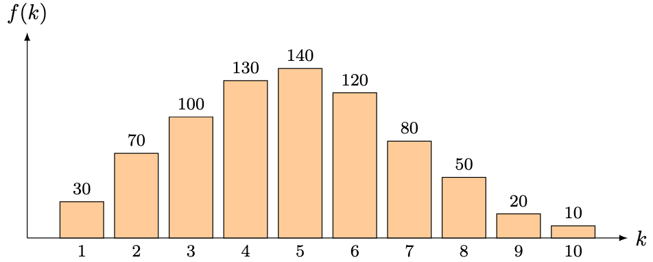
Problem 4 (Goodness-of-Fit). A total of 750 students took an assessment worth marks. For each , let denote the number of students who scored marks out of 10. We have the following data:
Assuming that scores are continuous, determine at the 5% significance level if the scores can be well-approximated using a normal distribution.
(Click for Solution)
Solution. Let denote the score of a randomly chosen student with and . We first set up the null and alternative hypotheses:
We first estimate and using and respectively. Denoting the scores by , the summary statistics are
Hence,
Now we assume holds, so that . Denoting
we will use the test statistic
which follows a -distribution with degrees of freedom. For a proof for why this distribution works, refer to this document. Using relevant -table look-up values (or a spreadsheet application), we obtain the following values for (rounded to the nearest integer for readability, but whose original value we use in the final computation):
Piecing all of the values together,
Using a -table, , which does not hold. Therefore, there is (woefully) insufficient evidence to reject and we cannot conclude that does not follow a normal distribution.
Problem 5 (Population Variance). Using the data in Problem 4, and assuming that the scores are normally distributed, test at the 5% significance level to determine if the standard deviation of assessment scores is greater than 2.
(Click for Solution)
Solution. We first set up the null and alternative hypotheses:
We use the test statistic :
Using a spreadsheet application, . Therefore, there is sufficient evidence to reject and conclude that , which implies .


![\mu = \mathbb E[X]](https://s0.wp.com/latex.php?latex=%5Cmu+%3D+%5Cmathbb+E%5BX%5D&bg=ffffff&fg=000&s=0&c=20201002)


.
.


![p := \mathbb E[\xi]](https://s0.wp.com/latex.php?latex=p+%3A%3D+%5Cmathbb+E%5B%5Cxi%5D&bg=ffffff&fg=000&s=0&c=20201002)


Leave a comment