Now that we have motivated the definitions of 


Lemma 1. For any 
Proof. The case 


so that 

If you are thinking that the sum-of-squares formula feels like déjà-vu, you are not wrong. The equation 


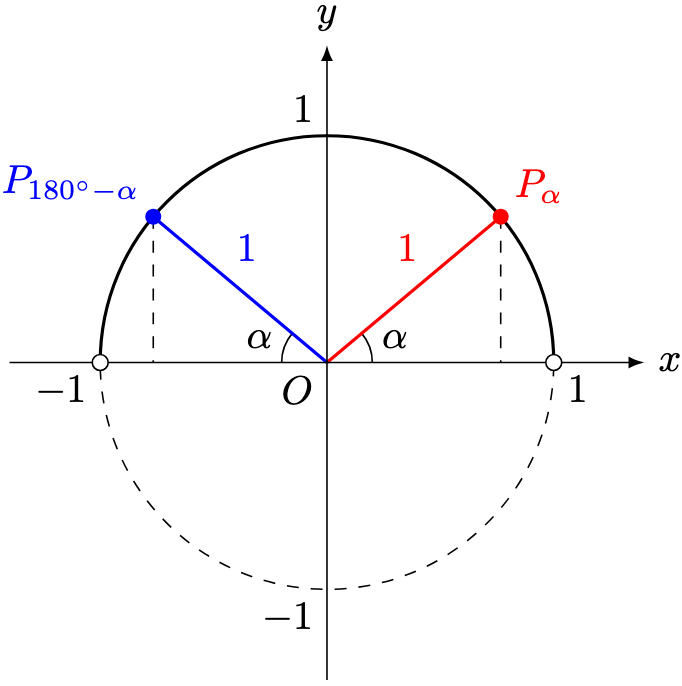
Furthermore, by measuring the clockwise angle relative to the positive 


Hence, we generalise for any 

When 

Therefore, we can extend the definitions of 

Definition 1. For any 
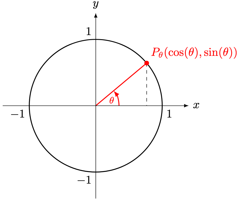
Define 
This definition agrees with the usual definitions of 
Example 1. Let

in terms of

Solution. We annotate on the usual unit circle diagram.
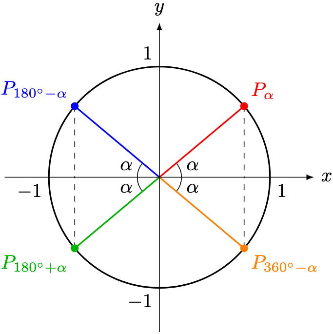
We can then deduce that

Similarly,

Remark 1. From this point onward, we will switch our discussions to “radian mode”, given by the conversion 

We will soon discuss calculus, which requires angles to be measured in radians.
Example 2. Evaluate 

Solution. Using Remark 1,

Example 3. Derive the definition of 

Solution. Firstly, for 

Since 


Furthermore, we remark that 


This post is titled applied trigonometry, but so far, we haven’t applied it in any meaningful sense. Not yet, at least.
The key is that since we have already defined 


Hence, we can divvy-up the interval 


Returning to the unit circle, there is no reason to restrict our graph to 


Hence, we can extend the definitions of
Definition 2. For any integer 


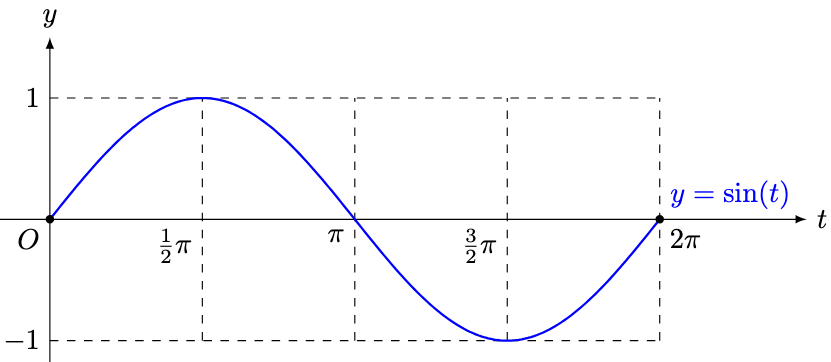
Now our complete graph for
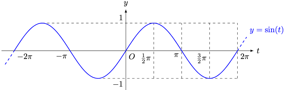
If this shape looks familiar to the waves that you see on the seaside, once again, you’re not wrong! These wavy shapes are called sinusoids, or more informally, sine waves. We will call the graph of
The most general form of a sine wave looks like 
Theorem 1. Define the sine wave 


- For any real
.
- The sine wave first repeats itself after a time interval of
.
- The roots of the sine wave are given by
, where
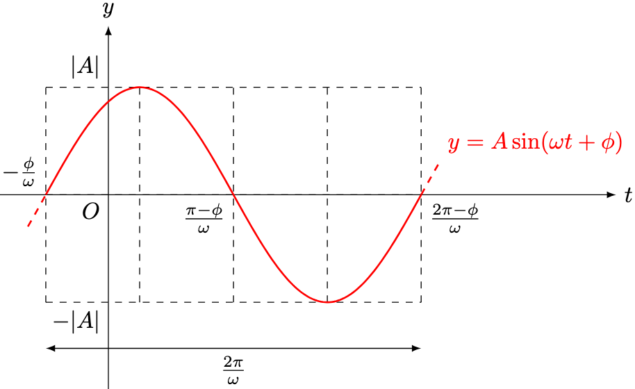
In this case, we give the constants the following names:
is the amplitude of the sine wave,
is the angular frequency of the sine wave,
is the leftward phase shift of the sine wave,
Proof Sketch. One cycle of the graph is obtained by the inequality

We calculated the special points using

where 
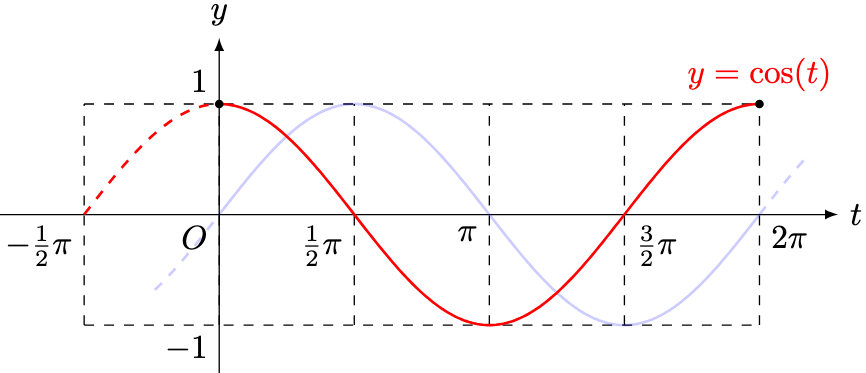
Example 4. Using Theorem 1, sketch the graph of 
Solution. Using the complementary and obtuse angle identities, if 

It can be shown that this identity holds for any real
- amplitude
- period
- leftward phase shift of
.
Hence, we sketch 
Therefore, for simplicity, we can just work with sine waves.
What happens when two waves 

Theorem 2. Let 
In particular, given positive constants 

where 

Proof. For the general case, see Problem 3 of this post. We will prove the special case directly. Expand the right-hand side using the addition formula:

Setting 


Using the Pythagorean identity,

Furthermore,

A direct proof is possible but far more cumbersome, and not terribly helpful for our discussions.
Sine waves are responsible for Fourier series that make modern electronics possible in the first place, so if you intend to explore electronics, you will find them helpful.
What we have discussed up to this point covers much of pre-calculus. What lies ahead seems tricky for many but turns out to be one of the most versatile branches of high school mathematics with respect to further studies in college and university—calculus.
We will explore calculus from a computational point of view, rather than explore its rich underlying theory. That exploration can take us down a very, very deep rabbit hole called real analysis, which we shall relegate as an ambitious exercise for a select subset of students.
For now, we shall turn to the first idea of our consideration: differentiation.
—Joel Kindiak, 20 Dec 25, 1240H

Leave a comment