Stationary Points

Differentiation finds one of its greatest powers in optimisation; that is maximising or minimising some constrained quantity.

Consider the graph of $y = f(x)$ below with minimum point $P(c, f(c))$ .

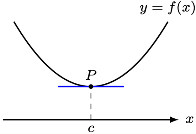
Since the tangent to the curve at $P$ is horizontal, it has a gradient of zero. That is, $f'(c) = 0$ .

Theorem 1 (Zero Derivative Condition). If $(c, f(c))$ is a local minimum or local maximum, then $f'(c) = 0$ . Denoting $y = f(x)$ ,

$\displaystyle \frac{\mathrm d y}{\mathrm dx} \Big|_{x = c} \equiv f'(c) = 0.$

Proof. We illustrate the proof for the local minimum case.

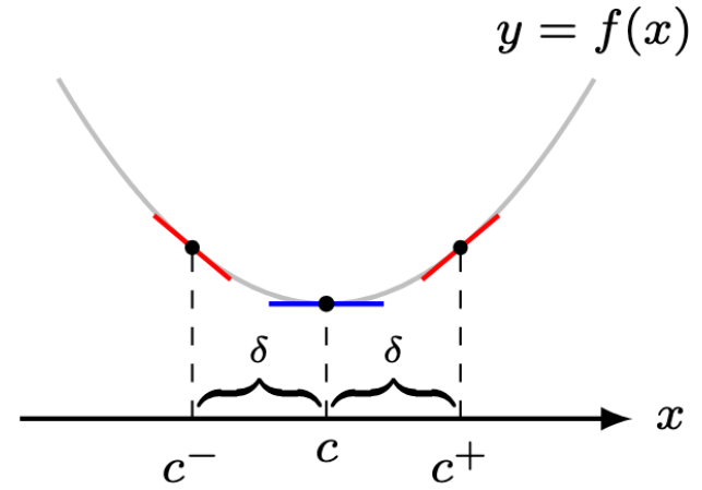
Denote $c^- = c-\delta$ and $c^+ = c+\delta$ for sufficiently small $\delta$ . The rough idea is that using the diagram,

$f'(c^-) < 0 < f'(c^+)$

so that by taking $\delta \approx 0$ ,

$f'(c) \leq 0 \leq f'(c) \quad \Rightarrow \quad f'(c) = 0.$

For more rigorous details, see this post.

Example 1. Calculate the turning points of the graph of $y = \frac 13x^3 - 4x + 2$ .

Solution. To determine the turning points, we use the zero derivative condition:

$\displaystyle \frac{\mathrm dy}{\mathrm dx} = 0.$

We first evaluate the left-hand side:

$\begin{aligned} \frac{\mathrm dy}{\mathrm dx} &= \frac{\mathrm d}{\mathrm dx} \left( \frac 13x^3 - 4x + 2 \right) \\ &= \frac 13 \cdot \frac{\mathrm d}{\mathrm dx}(x^3) - 4 \cdot \frac{\mathrm d}{\mathrm dx}(x) + \frac{\mathrm d}{\mathrm dx}(2) \\ &= \frac 13 \cdot 3x^2 - 4 \cdot 1 + 0 \\ &= x^2 - 4.\end{aligned}$

Hence, we solve the equation

$\begin{aligned} x^2 - 4 &= 0 \\ x^2 &= 4 \\ x &= \pm 2. \end{aligned}$

And we resolve two cases:

At $x = -2$ , $y = \frac 13 \cdot (-2)^3 - 4 \cdot (-2) + 2 = 22/3$ .
At $x = 2$ , $y = \frac 13 \cdot 2^3 - 4 \cdot 2 + 2 = -10/3$ .

Therefore, the two turning points have coordinates $(-2, 22/3)$ , $(2,-10/3)$ .

Remark 1. Using software, the graph of $y = \frac 13x^3 - 4x + 2$ is given as follows.

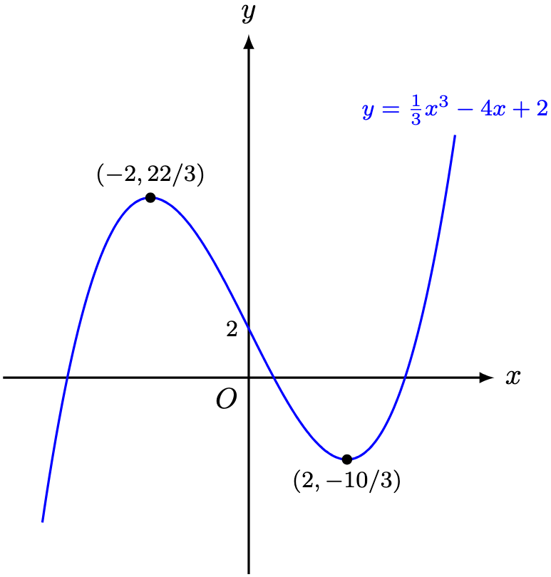
Hence, the power of calculus arises in calculating the turning points even without technology or visual intuition.

Example 2. Given constants $a,b,c,d$ with $a \neq 0$ , show that the graph

$y = ax^3 + bx^2 + cx + d$

has two distinct stationary points if and only if $b^2 - 3ac > 0$ .

Solution. We take the first derivative:

$\displaystyle \frac{\mathrm dy}{\mathrm dx} = 3ax^2 + 2bx + c.$

By the zero derivative condition, the graph has two distinct stationary points if and only if the equation $\displaystyle \frac{ \mathrm dy }{ \mathrm dx } = 0$ has two real and distinct roots. Now the equation

$3ax^2 + 2bx + c = 0$

has two real and distinct roots if and only if its discriminant is positive:

$\begin{aligned} (2b)^2 - 4 \cdot 3a \cdot c &> 0 \\ 4b^2 - 4 \cdot 3ac & > 0 \\ 4 \cdot (b^2 - 3ac) & > 0 \\ b^2 - 3ac & > 0. \end{aligned}$

Each step holds bi-directionally so the proof holds.

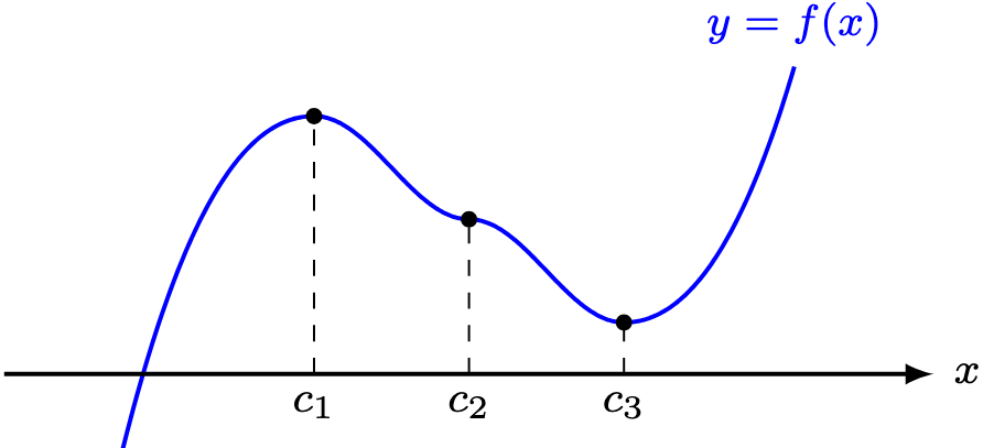
Suppose now we know that $f'(c) = 0$ . How do we know what kind of turning point $(c, f(c))$ is? Sadly, there is a third situation in which $f'(c) = 0$ .

By considering the graph above, there are three instances in which $f'(c) = 0$ occurs:

$c=c_1$ : at a local maximum,
$c=c_2$ : at a stationary point of inflection,
$c=c_3$ : at a local minimum.

How do we distinguish between these three types? Graphically, but expressed in equations.

Theorem 2 (First Derivative Test). Suppose $f'(c) = 0$ . For small $\delta > 0$ , define $c^- := c - \delta$ and $c^+ := c + \delta$ . Suppose $f'(c^-) \neq 0$ and $f'(c^+) \neq 0$ . Then $P(c, f(c))$ is a:

local minimum if $f'(c^-) < 0$ and $f'(c^+) > 0$ ,
local maximum if $f'(c^-) > 0$ and $f'(c^+) < 0$ ,
stationary point of inflection if $f'(c^-) f'(c^+) > 0$ .

Proof. The diagram above illustrates all three scenarios. For details, see this post.

Example 3. Determine the nature of the turning points calculated in Example 1.

It turns out that we can take a short-cut to Theorem 1 by considering the second derivative, defined by the derivative of the first derivative:

$f''(x) := (f')'(x).$

For alternate notation, suppose $y = f(x)$ , then

$\begin{aligned} \displaystyle \frac{\mathrm d^2 y}{\mathrm dx^2} &\equiv \frac{\mathrm d^2 }{\mathrm dx^2}(y) \equiv \left( \frac{\mathrm d}{\mathrm dx} \right)^2(y) \equiv \frac{\mathrm d}{\mathrm dx}\left( \frac{\mathrm d}{\mathrm dx}(y)\right) \equiv \frac{\mathrm d}{\mathrm dx}\left( \frac{\mathrm dy}{\mathrm dx} \right). \end{aligned}$

In turn, we have

$\begin{aligned} \frac{\mathrm d}{\mathrm dx}\left( \frac{\mathrm dy}{\mathrm dx} \right) = \frac{\mathrm d}{\mathrm dx}(f'(x)) = (f')'(x) = f''(x). \end{aligned}$

Theorem 3 (Second Derivative Test). Suppose $f'(c) = 0$ . Then $P(c, f(c))$ is a:

local minimum if $f''(c) > 0$ ,
local maximum if $f''(c) < 0$ .

If $f''(c) = 0$ , no conclusion can be made.

Proof Sketch. In the case of a local minimum,

$f'(c^-) < 0,\quad f'(c^+) > 0.$

Since $f''(c) = (f')'(c)$ measures the gradient of $y = f'(c)$ , and $f'$ is increasing from negative to positive, $f''(c) > 0$ . The local maximum case follows similarly. For rigour and detail, see this post.

Example 4. Calculate the stationary points of the graph $y = x + 1/x$ , $x \neq 0$ , and determine their nature.

Solution. To obtain the stationary points of the graph, we use the zero derivative condition

$\displaystyle \frac{\mathrm dy}{\mathrm dx} = 0.$

Evaluating the left-hand side,

$\begin{aligned} \frac{\mathrm dy}{\mathrm dx} &= \frac{\mathrm d}{\mathrm dx} \left( x + \frac 1x \right) \\ &= \frac{\mathrm d}{\mathrm dx}(x) + \frac{\mathrm d}{\mathrm dx} \left( \frac 1x \right) \\ &= 1 + \left( -\frac 1{x^2} \right) \\ &= 1 - \frac 1{x^2}. \end{aligned}$

Therefore, we solve the equation

$\begin{aligned} 1 - \frac 1{x^2} &= 0 \\ 1 &= \frac 1{x^2} \\ x^2 &= 1 \\ x &= \pm 1. \end{aligned}$

Now $y(1) = 1+1/1 = 2$ and $y(-1) = -1 + 1/(-1) = -2$ . Therefore, the stationary (not necessarily turning!) points are given by $(1, 2)$ and $(-1, -2)$ .

To determine their nature, we use the second derivative test:

$\begin{aligned} \frac{\mathrm d^2 y}{\mathrm dx^2} &= \frac{\mathrm d}{\mathrm dx} \left( \frac{\mathrm dy}{\mathrm dx} \right) \\ &= \frac{\mathrm d}{\mathrm dx} \left( 1 - \frac 1{x^2} \right) \\ &= \frac{\mathrm d}{\mathrm dx} ( 1 - x^{-2} ) \\ &= \frac{\mathrm d}{\mathrm dx}(1) - \frac{\mathrm d}{\mathrm dx} (x^{-2}) \\ &= 0 - ( -2x^{-2-1} ) \\ &= 2x^{-3} = \frac{2}{x^3}. \end{aligned}$

Using the second derivative test,

$\begin{aligned} \frac{\mathrm d^2 y}{\mathrm dx^2} \Big|_{x = 1}= \frac{2}{1^3} = 2 > 0,\quad \frac{\mathrm d^2 y}{\mathrm dx^2} \Big|_{x = -1}= \frac{2}{(-1)^3} = -2 < 0. \end{aligned}$

Therefore, $(1, 2)$ is a local minimum while $(-1, -2)$ is a local maximum.

Example 5. The diagram below shows the graphs of

$y = x^3,\quad y = x^4,\quad y = -x^4$

respectively.

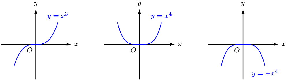
For each graph, compute $\displaystyle \frac{\mathrm d y}{\mathrm dx}$ and $\displaystyle \frac{\mathrm d^2 y}{\mathrm dx^2}$ at $x = 0$ . What do you notice?

Solution. For the first graph,

$\displaystyle y = x^3,\quad \frac{\mathrm dy}{\mathrm dx} = 3x^2,\quad \frac{\mathrm d^2 y}{\mathrm dx^2} = 6x.$

Therefore,

$\displaystyle \frac{\mathrm dy}{\mathrm dx}\Big|_{x = 0} = 3 \cdot 0^2 = 0 ,\quad \frac{\mathrm d^2 y}{\mathrm dx^2}\Big|_{x = 0} = 6 \cdot 0 = 0.$

For the first graph,

$\displaystyle y = x^4,\quad \frac{\mathrm dy}{\mathrm dx} = 4x^3,\quad \frac{\mathrm d^2 y}{\mathrm dx^2} = 12x^2.$

Therefore,

$\displaystyle \frac{\mathrm dy}{\mathrm dx}\Big|_{x = 0} = 4 \cdot 0^3 = 0 ,\quad \frac{\mathrm d^2 y}{\mathrm dx^2}\Big|_{x = 0} = 12 \cdot 0^2 = 0.$

Similarly, in the case $y = -x^4$ ,

$\displaystyle \frac{\mathrm dy}{\mathrm dx}\Big|_{x = 0} = 0 ,\quad \frac{\mathrm d^2 y}{\mathrm dx^2}\Big|_{x = 0} = 0.$

Remark 2. The point of this exercise is to demonstrate that $f'(c) = 0$ tells us that $(c, f(c))$ is a stationary point, but $f''(c) = 0$ does not give us any meaningful information about the nature of $(c, f(c))$ . The latter could occur in all three types of stationary points.

Now, we can talk about constrained optimisation.

Example 6. Determine the smallest perimeter for a rectangle with area $1$ units².

Solution. Sketch the rectangle as follows.

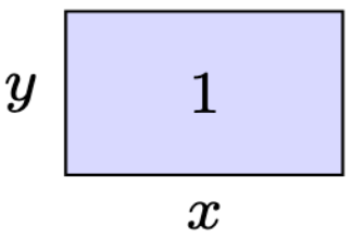
Since $xy = 1$ , we have $y = 1/x$ . Hence the rectangle has a total perimeter of

$\displaystyle P(x) = 2x + 2y = 2x + 2 \cdot \frac 1x = 2 \underbrace{ \left( x + \frac 1x \right) }_{f(x)}.$

Since $x > 0$ , $f(x) = x + 1/x > 0$ . Hence, $(c, P(c))$ is a local minimum if and only if $(c, f(c))$ is a local minimum. By Example 4, $(1, f(1))$ is a local minimum. Therefore, $(1, P(1)) = (1, 4)$ is a local minimum.

In particular, the smallest perimeter achieved is $4$ units², when $x = y = 1$ , i.e. the rectangle is a square with side length $1$ unit.

Remark 3. Strictly speaking, we need to do more work to show that $(1, 4)$ is a global minimum. However, in the context of high school mathematics, most problems uses expressions that do not need this extra technicality.

Example 7. Determine the smallest surface area for a closed cylinder with volume $10$ units³.

Solution. Sketch the cylinder as follows.

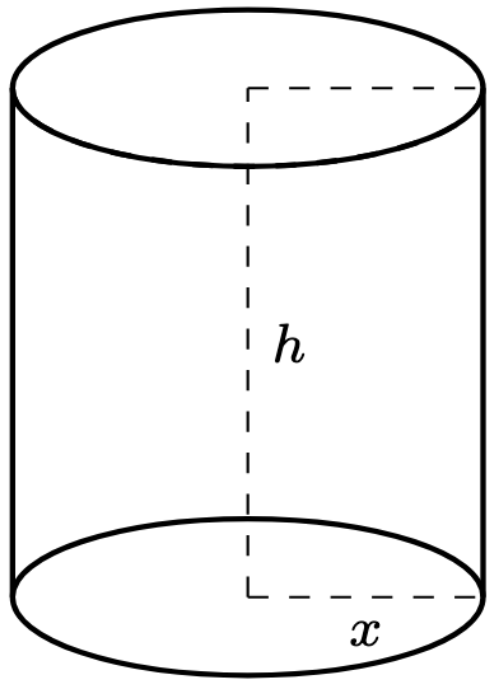
Here, $x > 0$ . Recalling the volume of a cylinder,

$\displaystyle \pi x^2 h = 10\quad \Rightarrow \quad h = \frac{10}{\pi x^2}.$

The surface area $A$ is made up of two circles with area $\pi x^2$ each and one curved surface with area $2 \pi x h$ . Hence,

$\begin{aligned} A(x) &= 2 \cdot \pi x^2 + 2 \pi x h \\ &= 2 \pi x^2 + 2 \pi x \cdot \frac{10}{\pi x^2} \\ &= 2 \pi x^2 + \frac{20}{x}. \end{aligned}$

To use the zero derivative condition, we first calculate $\displaystyle \frac{ \mathrm dA }{ \mathrm dx }$ :

$\begin{aligned} \frac{\mathrm dA}{\mathrm dx} &= \frac{\mathrm d}{\mathrm dx} \left( 2\pi x^2 + \frac{20}{x} \right) \\ &= 2\pi \cdot \frac{\mathrm d}{\mathrm dx} ( x^2 )+ 20 \cdot \frac{\mathrm d}{\mathrm dx}\left( \frac 1x \right) \\ &= 2\pi \cdot 2x + 20 \cdot \left( -\frac 1{ x^2 } \right) \\ &= 4 \left( \pi x - \frac 5{x^2} \right). \end{aligned}$

Hence, we set $\displaystyle \frac{ \mathrm dA }{ \mathrm dx } = 0$ :

$\begin{aligned} 4 \left( \pi x - \frac 5{x^2} \right) &= 0 \\ \pi x - \frac 5{x^2} &= 0 \\ \pi x &= \frac 5{x^2} \\ x^3 &= \frac 5{\pi}. \end{aligned}$

Therefore, $x = \sqrt[3]{5/\pi} \approx 1.17$ units. For the second derivative test, we calculate the second derivative:

$\begin{aligned} \frac{\mathrm d^2 A}{\mathrm dx^2} &= \frac{\mathrm d}{\mathrm dx} \left( \frac{\mathrm dA}{\mathrm dx}\right) \\ &= \frac{\mathrm d}{\mathrm dx} ( 4\pi x - 20 x^{-2} ) \\ &= 4\pi \cdot \frac{\mathrm d}{\mathrm dx} ( x ) - 20 \cdot \frac{\mathrm d}{\mathrm dx} (x^{-2}) \\ &= 4\pi \cdot 1 - 20 \cdot (-2)x^{-3} \\ &= 4\pi + 40 x^{-3} \\ &= 4\pi + \frac{ 40 }{ x^3 } > 0 \end{aligned}$

whenever $x > 0$ . By the second derivative test, $x = \sqrt[3]{5/\pi}$ yields a local maximum for $A$ :

$\begin{aligned} A &= 20 \pi x^2 + \frac{ 20 }{ x } \\ &= \frac 1{x} (2 \pi x^3 + 20 ) \\ &= \frac{ \sqrt[3]{\pi} }{ \sqrt[3]{5} } \left( 2\pi \cdot \frac 5{\pi} + 20\right) \\ &= \frac{ 30 \sqrt[3]{\pi} }{ \sqrt[3]{5} } \approx 25.7\, \text{units}^2. \end{aligned}$

While there are many possible applications of optimisation, especially in profit-maximisation, we want to switch gears and discuss differentiation’s shadow brother—integration. This we will computationally discuss next time.

For now, let’s resolve an interesting generalisation of the questions we solved just now.

Example 8. For positive constants $A, B$ , use calculus to show that

$\displaystyle \frac{A+B}{2} \geq \sqrt{AB}$

with equality if and only if $A = B$ .

Solution. Define the function $f(x) = Ax + B/x$ for $x > 0$ . Taking derivatives, we leave it as an exercise to check that

$\displaystyle f'(x) = A - \frac B{x^2},\quad f''(x) = \frac{2B}{x^3} > 0.$

By the zero derivative condition,

$\displaystyle f'(x) = 0 \quad \iff \quad x = \sqrt{ \frac BA }.$

Since $\sqrt{B/A} > 0$ , $f''(\sqrt{B/A}) > 0$ . By the second derivative test, $x = \sqrt{B/A}$ yields a local minimum at $f(\sqrt{B/A})$ :

$\displaystyle f(\sqrt{B/A}) = A \sqrt{\frac BA } + \frac{B}{\sqrt{B/A}} = 2\sqrt{A}\sqrt{B} = 2\sqrt{AB}.$

In particular, at $x = 1$ ,

$A + B = f(1) \geq f(\sqrt{B/A}) = 2\sqrt{AB}.$

Dividing by $2$ on both sides,

$\displaystyle \frac{A + B}{2} \geq \sqrt{AB}.$

Equality holds if and only if $\sqrt{B/A} = 1 \iff A = B$ .

Remark 4. The left-hand side $(A+B)/2$ is known as the arithmetic mean (AM) of $A,B$ . The right-hand side $\sqrt{AB}$ is known as the geometric mean (GM) of $A,B$ . Therefore, this result is known as the AM-GM inequality.

Remark 5. An alternative proof from just algebra arises from expanding the left-hand side of the not-so-trivial inequality

$(\sqrt A - \sqrt B)^2 \geq 0.$

—Joel Kindiak, 16 Jan 26, 1215H

KindiakMath

Stationary Points

Leave a comment Cancel reply

Stationary Points

Share this:

Leave a comment Cancel reply