Consider the following dot diagram that displays the heights, measured in cm, of 9 Gen Z humans.
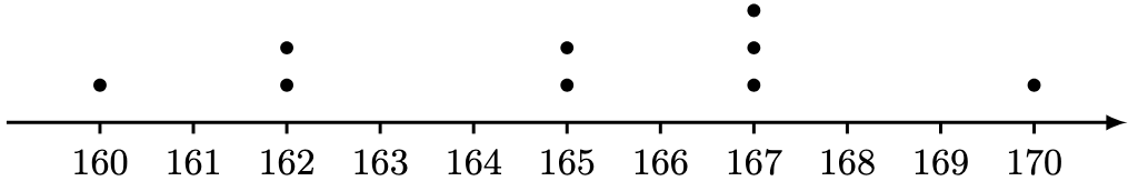
Question 1. What is the average height of these 9 individuals?
You might think that the answer is automatically obtained by adding all heights then dividing by 9. We will touch base with this kind of average later on. The problem is that the word “average” can take on multiple meanings.
One meaning means, what is the height that most people would have? Clearly, the height with the largest number of dots is 167 cm.
This means that the height that the majority of this set of 7 persons has is 167 cm. We call this the mode of the data set.
An element in a data set is called a data point.
Definition 1. The mode of a data set is the value taken on by majority of the data points.
We could formalise this notion using more technical symbols, but I don’t think that is helpful for us, since we are not terribly interested in any rigorous analysis of the data set.
Example 1. Consider the pie chart below illustrating the favourite music artists in 2025.
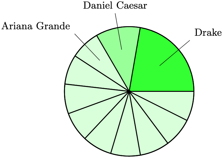
Then the most popular artist, namely Drake, is the mode of the data set. I am surprised that Taylor Swift isn’t on this list. Don’t flame me.
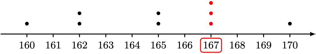
Example 2. Consider the dot diagram we started with.
According to the diagram, the mode of the data set is 167 cm. If, however, we add another data set at 162 cm, we get the dot diagram below.
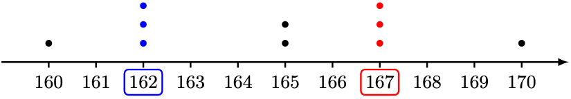
Then both 162 cm and 167 cm are modes of this data set. In this case, we call the data set bimodal.
This ambiguity could be a problem. We would like our answer to the “average” question to produce a unique answer.
To do that, we could interpret our data set as balancing on a beam with a pivot.
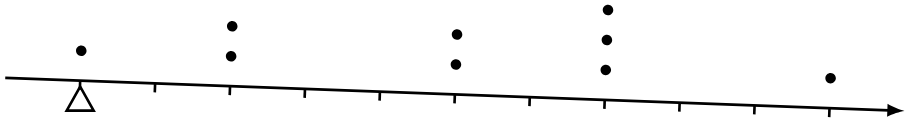
If the pivot is positioned at the 160 cm data point, then the entire beam would fall down. Likewise with the 170 cm data point.
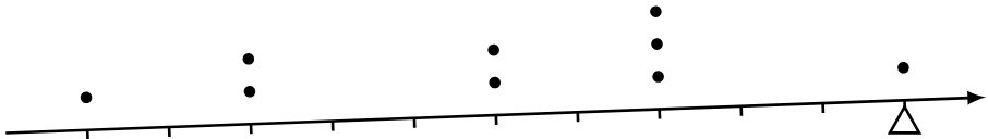
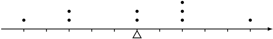
Question 2. Where would we position the pivot to balance the beam?
Intuitively, the further apart the data set is positioned from the pivot, the greater the rotating effect (i.e. the moment). Assume each data point has equal “mass”. Then we would like to compute some “balance point” 

Denoting the data set by 

Collecting the data points together,

By writing

where the Greek letter 

Definition 2. The mean of a data set 

Example 3. Consider the dot diagram we started with again.
By evaluating their sum, 
SUM(...). Hence, 
Example 4. Consider the same dot diagram, but now, a Gen Z human with height 140 cm is included.
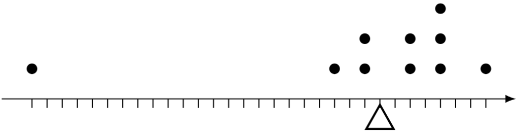
By evaluating their sum, 

Clearly, however, the 140 cm human is an exceptional case (i.e. an outlier) among this group of humans. However, since the mean incorporates all possible heights,
Question 3. Can we obtain an average that is less sensitive to outliers?
Return to the original data set.
If we arranged the data points in non-decreasing order, we obtain the following non-decreasing sequence:
160 ≤ 162 ≤ 162 ≤ 165 ≤ 165 ≤ 167 ≤ 167 ≤ 167 ≤ 170
In this ordered sense, the average height is 165 cm.
If we did include the outlier data point 140 cm, we get two middle values:
140 ≤ 160 ≤ 162 ≤ 162 ≤ 165 ≤ 165 ≤ 167 ≤ 167 ≤ 167 ≤ 170
In this latter case, the middle-of-the-middle is the simple average:

and the average height unchanged at 165 cm. We call this value the median height.
Definition 3. The median 

is defined by 


Using our data set, the median height remains unchanged when given the extra data point 140 cm. However, the median height can change; if instead we had an additional data point 190 cm, then we get two new middle values:
160 ≤ 162 ≤ 162 ≤ 165 ≤ 165 ≤ 167 ≤ 167 ≤ 167 ≤ 170 ≤ 190.
In this case, our new median is 
Intuitively, however, we would prefer the median to the mean for its relative resilience against outliers.
The mean and median have modifications that allow us to discuss the relative spread of data. We will explore this idea next time.
—Joel Kindiak, 9 Feb 26, 1346H

Leave a comment