Applied Integration

What was the point of integration? To compute areas. Which sounds strange. Don’t we already have meaningful formulas for common areas?

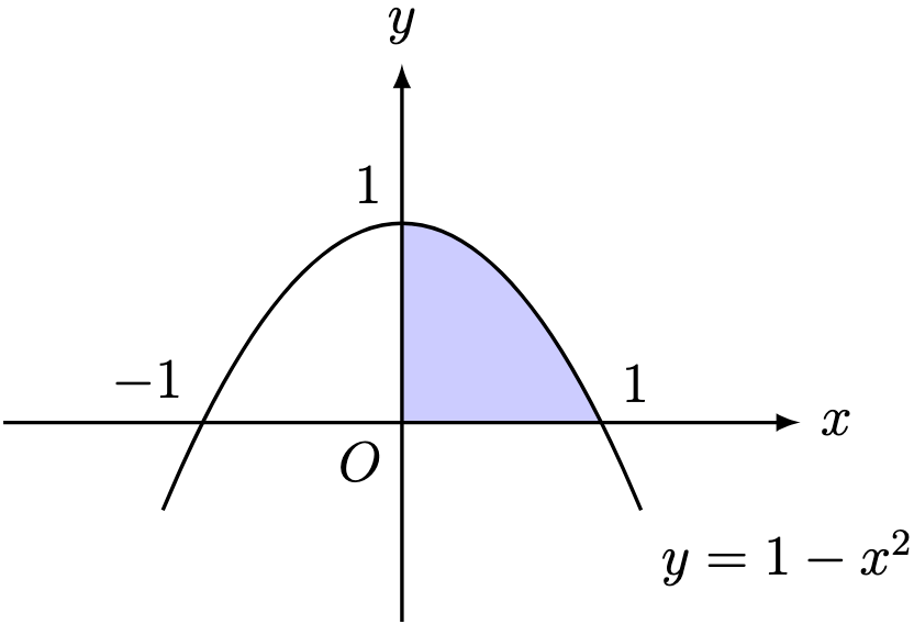
Example 1. Consider the graph $y = x$ below, with $0 < a < b$ .

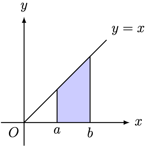
Define $F(x) = \displaystyle \int x\, \mathrm dx$ . Show that the shaded region has area

$F(b) - F(a).$

Solution. Using integration,

$F(x) = \displaystyle \int x\, \mathrm dx = \textstyle \frac{1}{2}x^2 + C.$

In particular,

$\begin{aligned} F(b) - F(a) &= \textstyle \left( \frac 12 b^2 + C \right) - \left( \frac 12 a^2 + C \right) \\ &= \textstyle \frac 12 b^2 - \frac 12 a^2. \end{aligned}$

Since the shaded region is a trapezium, it has an area given by

$\begin{aligned} (\text{area}) &= \textstyle \frac 12 \cdot (b+a) \cdot (b-a) \\ &= \textstyle \frac 12 \cdot (b^2 - a^2) \\ &= \textstyle \frac 12 b^2 - \frac 12 a^2 \\ &= F(b) - F(a). \end{aligned}$

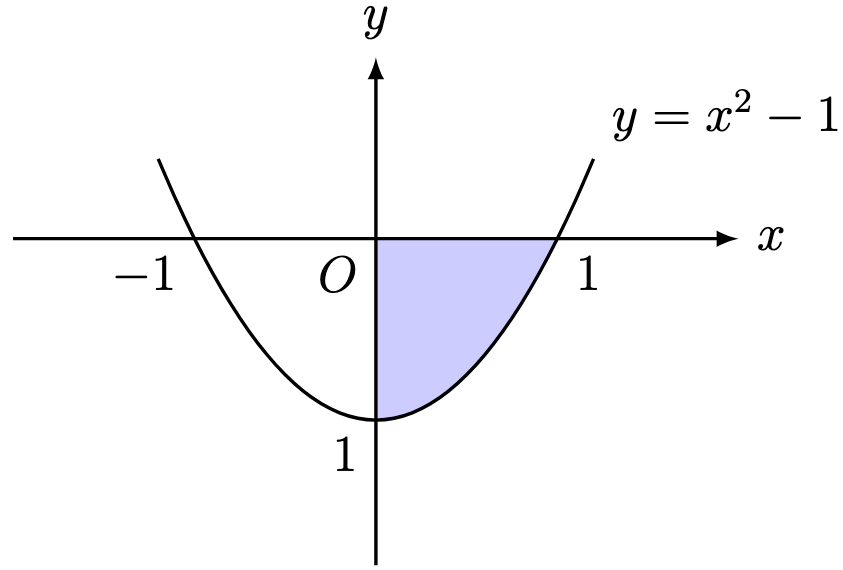
Example 2. Consider the graph $y = x^2$ below, with $b > 0$ .

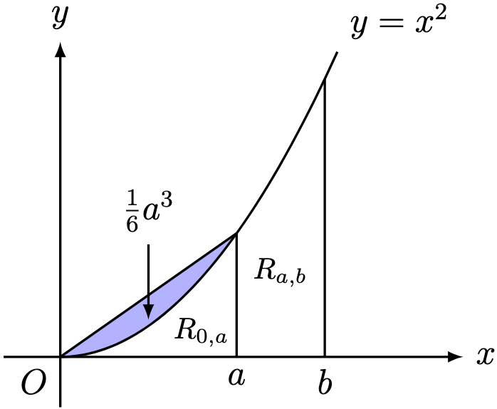
Define $\displaystyle F(x) = \int x^2\, \mathrm dx$ . The Greek mathematician Archimedes calculated the blue region to have an area of $\frac 16 a^3$ . Show that the area of $R_{0,a}$ is given by

$F(a) - F(0).$

Deduce that the area of $R_{a,b}$ is given by $F(b) - F(a)$ .

Solution. Using integration,

$F(x) = \displaystyle \int x^2\, \mathrm dx = \textstyle \frac{1}{3}x^3 + C.$

In particular, $F(a) - F(0) = \frac 13 a^3$ .

On the other hand, $R_{0,a}$ has area

$\begin{aligned} (\text{area of } R_{0,a}) &= \textstyle \frac 12 \cdot a \cdot a^2 - \frac 16 a^3 \\ &= \textstyle \frac 12 a^3 - \frac 16 a^3 \\ &= \textstyle \frac 13 a^3 = F(a) - F(0). \end{aligned}$

The region $R_{a,b}$ can be thought of as the “leftover” region of $R_{0,b}$ after removing $R_{0,a}$ , and hence has area

$(F(b) - F(0)) - (F(a) - F(0)) = F(b) - F(a).$

This pattern turns out to be true in more general settings. We will simply state this general pattern, and omit its proof (referencing it for more a more advanced study of calculus).

Theorem 1. Consider the graph $y = f(x)$ below, and suppose it lies above the $x$ -axis.

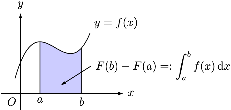
Define $F(x) = \displaystyle \int f(x)\, \mathrm dx$ . Then the area of the shaded region is given by

$\displaystyle F(b) - F(a).$

Proof. This result is known as the famous fundamental theorem of calculus, which is rigorously proven elsewhere in the blog.

Definition 1. Given any function $G(x)$ , make the notation

$[G(x)]_a^b := G(b) - G(a).$

Suppose we know the functions $f(x), F(x)$ such that

$\displaystyle F'(x) = f(x) \quad \iff \quad \int f(x)\, \mathrm dx = F(x) + C.$

Then we define the definite integral of $f(x)$ from $a$ to $b$ by

$\displaystyle \int_a^b f(x)\, \mathrm dx := [F(x)]_a^b \equiv F(b) - F(a).$

In particular, if $y = f(x)$ lies above the $x$ -axis, then

$\displaystyle \int_a^b f(x)\, \mathrm dx$

denotes the area of the region in Theorem 1.

Example 3. For $n \neq -1$ , evaluate $\displaystyle \int_0^1 x^n\, \mathrm dx$ .

Solution. Using integration,

$\displaystyle \int x^n\, \mathrm dx = \frac{x^{n+1}}{n+1} +C.$

Hence,

$\displaystyle \int_0^1 x^n\, \mathrm dx = \left[ \frac{x^{n+1}}{n+1} \right]_0^1 = \frac{1^{n+1}}{n+1} - \frac{0^{n+1}}{n+1} = \frac 1{n+1}.$

More generally, for any real $t$ ,

$\displaystyle \int_0^t x^n\, \mathrm dx = \frac {t^{n+1}}{n+1}.$

Using the definition of the definite integral, we can recover several important integration properties.

Theorem 2. Let $a,b,c,\alpha$ be real constants with $a \leq b \leq c$ . Whenever well-defined, the following definite integral properties hold:

$\begin{aligned} \int_a^b(f(x)+g(x))\, \mathrm dx &= \int_a^b f(x)\, \mathrm dx + \int_a^b g(x)\, \mathrm dx, \\ \int_a^b(\alpha \cdot f(x))\, \mathrm dx &= \alpha \cdot \int_a^b f(x)\, \mathrm dx, \\ \int_a^c f(x)\, \mathrm dx &= \int_a^b f(x)\, \mathrm dx + \int_b^c f(x)\, \mathrm dx, \\ \int_a^a f(x)\, \mathrm dx &= 0, \\ \int_b^a f(x)\, \mathrm dx &= -\int_a^b f(x)\, \mathrm dx. \end{aligned}$

Proof. We will prove just the third result and relegate the rest of the results as exercises. Suppose $F(x)$ satisfies

$\displaystyle F(x) = \int f(x)\, \mathrm dx.$

Then

$\begin{aligned} \int_a^b f(x) \, \mathrm dx + \int_b^c f(x) \, \mathrm dx &= [F(x)]_a^b + [F(x)]_b^c \\ &= (F(b) - F(a)) + (F(c) - F(b)) \\ &= F(c) - F(a) \\ &= \int_a^c f(x) \, \mathrm dx. \end{aligned}$

Example 4. Evaluate the exact area of the following region.

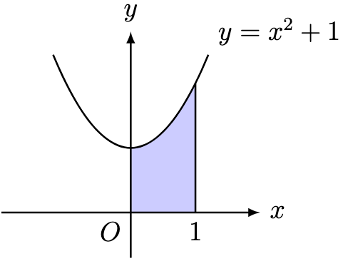
Solution. Since the area under the graph is calculated using an integral,

$\begin{aligned}(\text{area}) &= \int_0^1(x^2 + 1)\, \mathrm dx \\ &= \int_0^1 x^2\, \mathrm dx + \int_0^1 x^0\, \mathrm dx \\ &= \frac 1{2+1} + \frac 1{0+1} \\ &= \frac 43\, \text{units}^2.\end{aligned}$

Remark 1. Paradoxically, a rigorous treatment of calculus first proves Theorem 2 using a more fundamental definition of integration, then uses Theorem 2 and other real-analytic tools to prove Theorem 1.

Remark 2. The theory of integration is an incredibly deep rabbit hole, arguably deeper than that of differentiation. Its uses are deep and far-reaching due to its connections with probability (which influences basically almost every area of life). However, to keep things simple, we will restrict our attention to simple computations of integrals.

The rest of this post could evolve into a mere hodge-podge of integration drills, but perhaps we can think about Theorem 1 a little more closely.

Example 5. Consider the graph of $y = 1-x^2$ below.

Evaluate $\displaystyle \int_0^1 (1 - x^2)\, \mathrm dx$ and $\displaystyle \int_0^1 (x^2 - 1)\, \mathrm dx$ .

Solution. Using the linearity of integration

$\begin{aligned} \int_0^1(1-x^2 )\, \mathrm dx &= \int_0^1 x^0\, \mathrm dx - \int_0^1 x^2\, \mathrm dx \\ &= \frac 1{0+1} - \frac 1{2+1} \\ &= \frac 23.\end{aligned}$

By Theorem 2,

$\begin{aligned} \int_0^1(x^2 - 1)\, \mathrm dx &= -\int_0^1(1-x^2 )\, \mathrm dx = -\frac 23.\end{aligned}$

If, instead, we graphed $y = x^2 - 1$ , the corresponding shaded region would lie below the $x$ -axis.

Furthermore, it would have an area of $2/3$ units².

Hence, strictly speaking, the integral only accounts for the signed area, which is positive if $y = f(x)$ lies above the $x$ -axis, and negative if $y = f(x)$ lies below the $x$ -axis.

In many ways, integration was formulated to answer problems in physics.

Definition 2. Sir Isaac Newton used calculus to formulate the connections between displacement $s(T)$ , velocity $v(T)$ , and acceleration $a(T)$ at time $T$ as follows:

$\begin{aligned} s(T) &:= s(0) + \int_0^T v(t)\, \mathrm dt, \\ v(T) &:= v(0) + \int_0^T a(t)\, \mathrm dt. \end{aligned}$

We remark that these definitions agree with the usual velocity-time graph (for displacement) and the acceleration-time graph (for velocity), where we calculate the desired quantities by evaluating the areas under the graphs (hence, corresponding with the integral formulation)

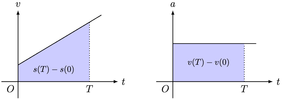
He was interested in the special case when $a(t)$ is a constant number, namely $a(t) \approx -9.81 =: g$ , known as the gravitational acceleration near the surface of Earth.

Theorem 3. Given constants $s_0, v_0, a_0$ , suppose

$s(0) = s_0, \quad v(0) = v_0, \quad a(t) = a_0$ .

Then

$v(T) = v_0 + a_0 T, \quad s(T) = s_0 + v_0 T + \frac 12 a_0 T^2.$

Furthermore, $v(T)^2 = v_0^2 + 2a_0 \cdot (s(T) - s_0)$ .

Proof. Integrating $a(t)$ ,

$\displaystyle \int a(t)\, \mathrm dt = \int a_0\, \mathrm dt = a_0t + C.$

Therefore,

$\begin{aligned} v(T) &= v(0) + \int_0^T a(t)\, \mathrm dt \\ &= v_0 + [a_0x]_0^T \\ &= v_0 + (a_0 T - a_0 \cdot 0) \\ &= v_0 + a_0T. \end{aligned}$

Similarly,

$\begin{aligned} \int v(t)\, \mathrm dt &= \int (v_0+a_0t)\, \mathrm dt \\ &= \int v_0\, \mathrm dt + a_0 \int t\, \mathrm dt \\ &= (v_0t + C_1) + \left(a_0 \cdot \frac{t^2}{2} + C_2 \right) \\ &= \textstyle v_0t + \frac 12 a_0t^2 + C, \end{aligned}$

where $C := C_1 + C_2$ . Therefore,

$\begin{aligned} s(T) &= s(0) + \int_0^T v(t)\, \mathrm dt \\ &= \textstyle s_0 + \left[ v_0t + \frac 12 a_0t^2 \right]_0^T \\ &= \textstyle s_0 + \left( v_0T + \frac 12 a_0T^2 \right) - \left( v_0\cdot 0 + \frac 12 a_0 \cdot 0^2 \right) \\ &= \textstyle s_0 + v_0T + \frac 12 a_0T^2 . \end{aligned}$

In particular,

$\begin{aligned} v(T)^2 &= ( v_0 + a_0T )^2 \\ &= \textstyle v_0^2 + 2v_0a_0T + a_0^2 T^2 \\ &= \textstyle v_0^2 + 2a_0 {\left( v_0T + \frac 12 a_0 T^2 \right)} \\ &= v_0^2 + 2a_0 \cdot (s(T) - s_0). \end{aligned}$

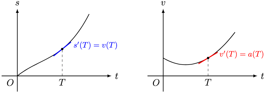
Theorem 3 lists out several common laws of kinematics, in particular, for an object moving in a straight line at constant acceleration. If instead we started by knowing the displacement $s(t)$ , we can recover the velocity and acceleration of the particle using differentiation.

Theorem 4. The displacement $s(t)$ , velocity $v(t)$ , and acceleration $a(t)$ of a particle moving in a straight line are related by the equations:

$\displaystyle v(t) = \frac{\mathrm ds}{\mathrm dt},\quad a(t) = \frac{\mathrm dv}{\mathrm dt}.$

In particular, $\displaystyle a(t) = \frac{\mathrm d^2 s}{\mathrm dt^2}$ . This connection arises ubiquitously in physics due to Newton’s second law.

Proof. Write $\displaystyle F(x) = \int v(x)\, \mathrm dx$ so that $F'(x) = v(x)$ and

$s(t) = s(0) + F(t) - F(0).$

Differentiating on both sides,

$\begin{aligned} \frac{\mathrm ds}{\mathrm dt} = \frac{\mathrm d}{\mathrm dt}(s(t)) &= \frac{\mathrm d}{\mathrm dt}(s(0) + F(t) - F(0)) \\ &= \frac{\mathrm d}{\mathrm dt}(s(0)) + \frac{\mathrm d}{\mathrm dt}(F(t)) - \frac{\mathrm d}{\mathrm dt}(F(0)) \\ &= 0 + F'(t) - 0 \\ &= F'(t) \\ &= v(t). \end{aligned}$

The argument holds similarly for $a(t)$ .

Similarly, these connections agree with the usual displacement-time graph (for velocity) and the velocity-time graph (for acceleration), where we calculate the desired quantities at a specific time by evaluating the gradient of the tangent at that point.

We have only scratched the surface regarding applied calculus, and you can explore even more in adjacent STEM fields like physics and economics.

For now, we need to answer a crucial question. So far, we have only discussed calculus regarding the simple-enough polynomials. But can we discuss calculus on the trigonometric functions like $\sin(x)$ and $\cos(x)$ , and the exponential family $e^x$ and $\ln(x)$ of functions?

The answer is yes, sort of. A rigorous treatment takes a lot more effort into the nuts and bolts of calculus. Nevertheless, we can still appreciate these formulas from a visually intuitive perspective, and I think there is still a lot to enjoy from viewing it that way.

—Joel Kindiak, 23 Jan 26, 1937H

KindiakMath

Applied Integration

Leave a comment Cancel reply

Applied Integration

Share this:

Leave a comment Cancel reply