The three-dimensional version of “area” and “perimeter” would be, rather unsurprisingly, “volume” and “surface area”.
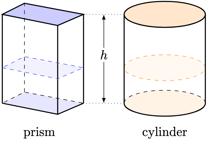
We start with the simplest object: a prism.
Definition 1. A solid with height is called a prism if all of its cross-sections have the same shape. In the special case that the base of the prism is a circle, we call the solid a cylinder.
Just like how a rectangle has area , a prism also has volume
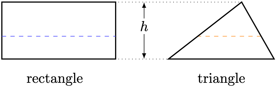
In that sense, a prism is similar to a “three-dimensional” rectangle, with many possible shapes for its base.
Corollary 1. The volume of a cylinder with height and base radius is .
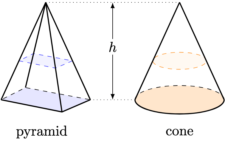
If there’s a “three-dimensional” rectangle, is there a “three-dimensional” triangle? Yes, and it’s called a pyramid.
Definition 2. A solid with height is called a pyramid if all of its cross-sections are similar to one another, and they “shrink” to a common point. In the special case that the base of the prism is a circle, we call the solid a cone.
This description is similar to that of a triangle: the bases are similar to one another and “shrink” to a common point:
We have seen that a triangle has area . What’s the formula for that of a pyramid?
Theorem 1. The volume of a prism is .
Proof. Omitted as it requires integral calculus. Nevertheless, the factor is directly related to the dimensions in which we defined a pyramid.
Corollary 2. The volume of a cone with height and base radius is .
Proof. By Theorem 1, the cone has a volume of
Having discussed volumes, it’s worth looking into its partner, surface areas. As the name suggests, surface areas refer to the areas of the surfaces of a solid. But what happens when weird faces abound?
We can’t discuss them all, but there are some special cases.
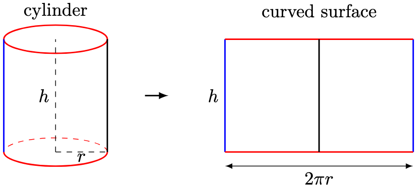
Theorem 3. The curved surface area of a cylinder with height and radius is .
Proof. The curved surface area of a cylinder can be thought of as a “wrap” of a rectangle with base and height :
Hence, the curved surface area is .
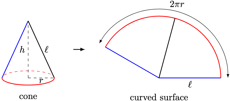
Theorem 4. The curved surface area of a cone with height and radius is .
Proof. Let denote the slant height of the cone. The curved surface area of a cone can be thought of as a “wrap” of a sector with radius :
Now the length of the arc of the sector is the circumference of the original cone, namely, . Hence, the total area of the sector is given by
Now by Pythagoras’ theorem,
Therefore, the curved surface area is , as required.
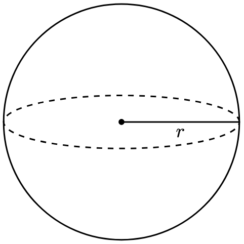
Finally we should discuss the geometry of the three-dimensional version of a circle: the sphere.
Definition 2. Define the sphere with centre and radius to be the set of points whose distance from the centre is .
Theorem 5. The volume of a sphere with radius is . The surface area of a sphere is .
Proof. Omitted as it requires integral (and arguably, differential) calculus.
Having developed the many commonly-used formulas in high school geometry, we cannot avoid the dreaded T-word: trigonometry. Contrary to popular anxiety, trigonometry is simply a new language to describe the relationship between straightedges and curves (i.e. angles). More on that in the next post.
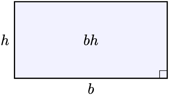
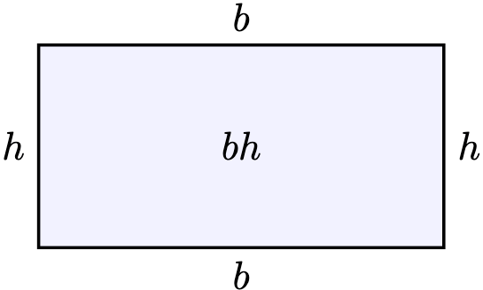
We start by considering the area of a rectangle. If a rectangle has base (units) long and height , its area is .
In fact, we used the rectangle intuition to list out the properties of real numbers, since we regarded as real numbers.
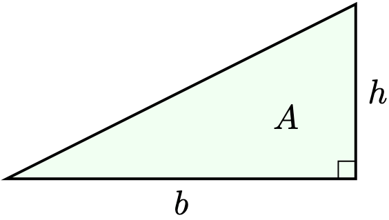
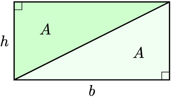
Theorem 1. Any triangle with base and height has area .
Proof. We first suppose the triangle is right-angled:
By duplicating the triangle and rotating it, we obtain a rectangle with base and height :
Denoting the area of the triangle by ,
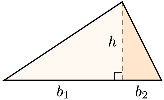
Now suppose the altitude lies inside the triangle:
Adding the areas, we obtain a total area of
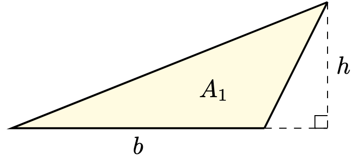
Now we consider the case when the altitude lies outside of the triangle:
Denote the area of the original triangle by . Consider the new triangle with area as follows:
Since areas are additive, use the first case to obtain
Performing algebruh,
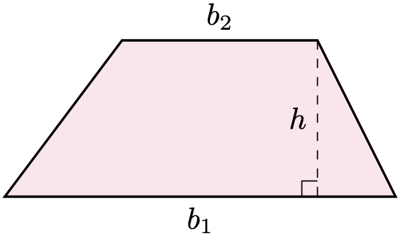
Theorem 2. Any trapezium with bases and height has area .
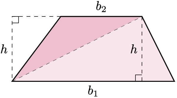
Proof. Consider the following trapezium without loss of generality:
Split the trapezium into two identical triangles:
Using Theorem 1, the area of the trapezium is given by
Theorem 3. Any parallelogram with base and height has area .
Proof. Consider the parallelogram below without loss of generality:
Since this parallelogram is a trapezium with bases , by Theorem 2, its area is given by
Most high school geometry problems boils down to applying these formulas one after another. However, they also include more “curvy” areas like circles. How do we compute such areas? We could memorise their formulas like , but how do we get that formula in the first place?
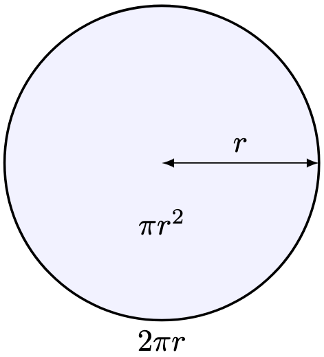
Definition 1. Given a circle with circumference and radius , we define to be the constant
Equivalently, we recover the circumference formula . Numerically, .
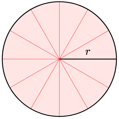
Theorem 4. The area of a circle with radius is .
Proof Sketch. We will subdivide the circle into a collection of “curved triangles” or more technically, sectors:
Here, we use sub-divisions for convenience. We notice that the areas total to the circle area. By rearranging these sectors, we recover an approximate rectangle with approximate base and approximate height :
Therefore, using the area of a rectangle, the circle has approximate area . Increasing the number of subdivisions improves the approximation, and in the limit, we get an exact area of .
Remark 1. A more complete construction can be formalised using integral calculus.
Finally, lets re-visit angles for completeness. Previously, we have usually used degrees— (i.e. degrees) to denote the angle of a “complete turn”. The reason for is convenience—the number has the factors that find many uses in astronomy and geology. In particular, denotes a -turn, denotes a -turn, so on and so forth.
Rather than use the convenience of , we might find it helpful to use the circumference of a circle. If a circle has radius , then its circumference is :
Here’s our intuition: an angle of denotes a complete turn. In particular, . In this case, we say that the angle is radians, and automatically refer to “radians” when we do not write any unit.
Definition 2. An angle is said to be of radians if the corresponding curved segment (i.e. arc) in the unit circle has a length of .
Therefore, an angle of radians corresponds to the whole circumference.
Lemma 1. Given any circle with radius , the angle corresponding to an arc with length is given by
Equivalently, . In particular, , agreeing with our prior intuitions on the circumference.
Proof Sketch. Consider the diagram below.
By regarding arcs as limits of straight lines, we can pass the intercept theorem for similar triangles to the limit and obtain
Therefore, radians work for angles regardless of radius size.
Lemma 2.. By algebra,
Here, of course, .
Theorem 5. A sector with radius and interior angle (radians) has area . In particular, with a full circle, we obtain the expected area .
Proof. Since the sector sweeps of the original circle, its area would correspond to
For a full circle, set to obtain an area of .
Having explored areas, we need to think deeper. Literally. Next time, we will look at volumes and surface areas, the three-dimensional version of areas and perimeters.
Oh, let’s just conclude with perimeters:
Definition 3. The perimeter of a shape is the total length of its boundary.
Example 1. A rectangle with base has perimeter :
Example 2. A circle with radius has perimeter :
Indeed, the perimeter of a circle is simply its circumference.
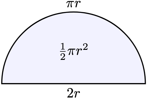
Example 3. A half-circle (i.e. a semicircle) with radius has perimeter :
This post isn’t about God; I write at length about God elsewhere.
We have explored expressions involving , and even binomials such as . Much of our exploration arises from interpreting powers as repeated multiplication in the following sense: given any positive number and positive integers ,
It turns out that we are allowed to regard as real numbers.
Theorem 1. Given any positive number , for real numbers ,
We call the base–exponential of .
Proof. The complete construction of the exponential takes place here, using the tools in undergraduate real analysis.
Theorem 2 (Laws of Exponents). Using the exponential in Theorem 1, we have the following laws of exponents:
Here, refers to a positive integer, and refers to real numbers.
Proof. Using Theorem 1,
Factorising ,
Similarly, by applying Theorem 1 a total of times,
Using Theorem 1 and the first result,
Finally, using Theorem 1 and the previous result,
Just like how we devoted nontrivial time and energy to solve equations that look like (it is ), we would also like to solve equations such as . We observe that, rather straightforwardly, if is an integer, then
However, how do we solve equations such as ? The idea is to use better and better decimal approximations of , and we give the “perfect” answer—the base-logarithm of . For a proper, technical construction, see the same post pertaining exponential functions.
Definition 1. Given real constants with , the base-logarithm of is the unique number such that
In this case, we denote .
Theorem 3 (Inverse Property). Given real constants with ,
Proof. Define . By Definition 1,
Similarly, define . By Definition 1,
Thanks to the basic property described in Theorem 1, the laws of exponents, and the inverse property, we recover all of the laws of logarithms. But to do that, we need our special friend .
Theorem 4. Given positive constants , we have the following laws of logarithms:
Furthermore , and for any ,.
Proof Sketch. We prove the first property, prove a special case for the last property, and relegate the others as an exercise in definition chasing. Using Theorem 1 and the inverse property,
By Definition 1, . For the last property, we prove the special case that is a positive integer:
The general case uses our technical definition of the exponential as outlined in the real-analysis posts.
Corollary 1. Given real constants and ,
Proof. Using the last property in the laws of logarithms,
By the inverse property,
as required.
Example 1. By considering the real number , demonstrate the existence of irrational numbers such that is rational. You may assume without proof that is irrational.
Solution. There are two cases to consider: either is rational or not. If is rational, then setting yields
which is rational. If is irrational, then setting and yields, by Corollary 1,
which is rational.
No matter which scenario is ultimately true, we can always arrive at the conclusion that there exist irrational numbers such that is rational.
Theorem 5 (Change-of-Base). Given positive numbers ,
In particular, denoting and , where denotes the exponential unit,
Proof. Using the inverse property,
The base- logarithm finds much use in numerically estimating the logarithms. For instance, the pH of a solution that measures the acidity of that solution (crucial in ecological applications) is defined by the number , where denotes the concentration of protons in that solution. The base- logarithm finds much use in theoretical analysis, since the rate of change of the function is .
Exponentials and logarithms form the cornerstone of any discussion involving rates of change, i.e. calculus, and infect every serious field of study in STEM: population growth in biology, cooling laws in thermodynamics, logistic growth in machine learning, so on and so forth.
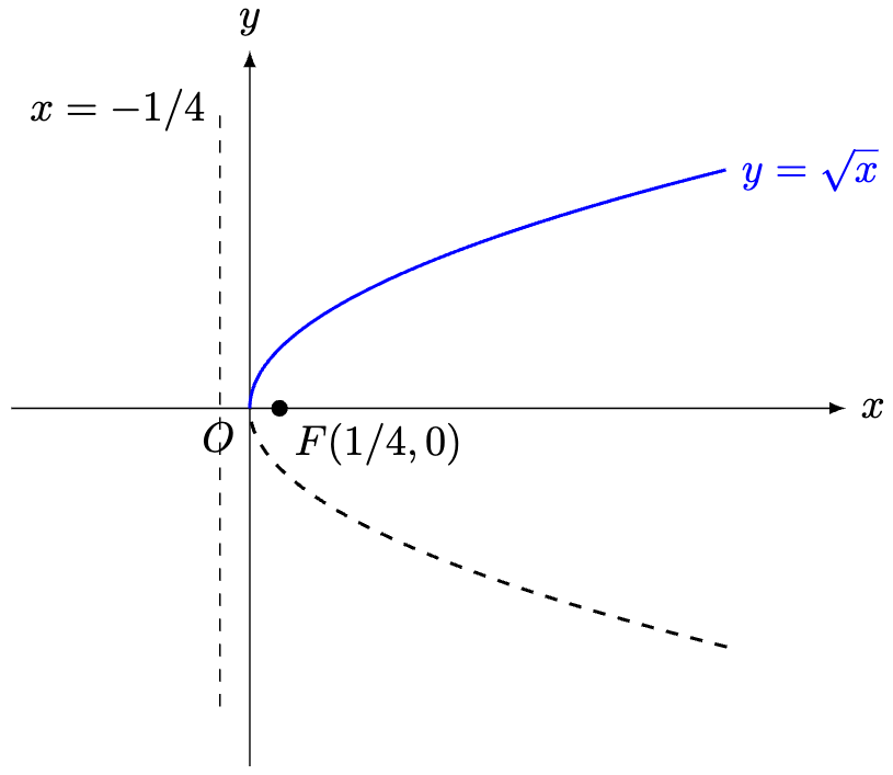
Previously, we have seen that given , the graph of looks like the diagram below.
For any point on the graph, it has the same distance to the (focal) point and the (directrix) line . Hence, its shape is known as a parabola. In particular, it has a minimum point .
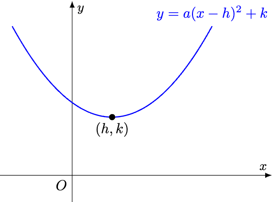
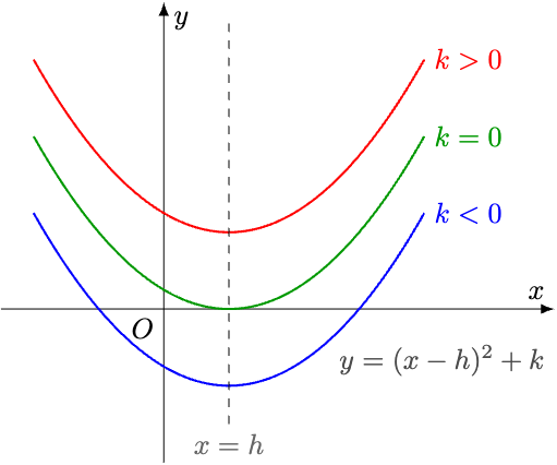
If we shifted the graph rightwards by and upwards by , we recover a more general parabola with minimum point .
Of course, if , then the whole graph gets “flipped” to the downside:
The diagram above shows the graph of .
Example 1. Determine the -intercept of the quadratic graph .
Solution. To determine the -intercept of the quadratic graph, we need to find the intersection of the graph and the -axis, whose equation is . Since the -values should match, we can substitute the latter equation into the former:
Therefore, our -intercept is . No surprises there.
Example 2. Determine the two -intercepts of the quadratic graph .
Solution. To determine the two -intercepts of the quadratic graph, we need to find the intersections of the graph and the -axis, whose equation is . Since the -values should match, we can substitute the latter equation into the former:
It is tempting at this stage to write so that our -intercept is . However, this solution is only partially correct. Just like any solution in Singapore or US politics.
Notice in the graph that we have a second-intercept to the left of the -axis. This is because could have been a negative number as well. Notice that
are both correct equations. (Furthermore, these are the only two correct equations). Therefore, if , we must conclude either possibility, namely, that or . To abbreviate, we use the notation: . This notation states that either or are plausible values that represents.
To answer our original question, since and in both cases, there are two -intercepts: and .
Example 3. Determine the -intercept(s) of the quadratic graph .
Solution. To determine the two -intercepts of the quadratic graph, we need to find the intersections of the graph and the -axis, whose equation is . Since the -values should match, we can substitute the latter equation into the former:
By Example 2, we have the solutions . Therefore, there are two -intercepts: and .
Remark 1. Different graphs can yield the same roots.
Example 4. Determine the -intercept(s) of the quadratic graph , where respectively.
Solution. We recall that . Therefore,
To find the -intercepts of the graph, we set :
Now we analyse this equation case-by-case.
If , then . Taking square roots,
Hence, or , yielding the -intercepts and .
If , then . Taking square roots,
Hence, or , yielding the -intercepts and .
If , then . Taking square roots,
Hence, , yielding only one -intercept .
If , then . Now, if is a real number, then is a real number too, which implies that . Therefore, . This can only mean that the equation has no real solutions, and therefore, the graph of no -intercepts.
The diagram below shows the graphs of all four cases.
Example 5. Given real numbers and , determine the number of -intercepts of the quadratic graph , and determine them in terms of and if they exist.
Solution. Repeating the calculations in Example 4, we set :
There are three cases: , , or .
In the case , , so that . Hence,
Therefore, the graph has two -intercepts and .
In the case ,
Therefore, the graph has only one -intercept .
In the case , , so that
Therefore, the equation has no real solutions, and the graph has no -intercepts.
Remark 2. The line is called the line of symmetry of the graph, and the point is the turning point of the graph.
Definition 1. We say that is a real numbersolution of the quadratic equation if . Equivalently,
is a real numbersolution of the equation,
is a root of the function,
is an -intercept of the graph .
Theorem 1. Let be a quadratic equation, where . Define the discriminant of the quadratic equation by
Then the equation has
real number solutions if ,
real number solution if , and
real number solutions if .
In the first two cases, the roots are given by the quadratic formula:
Proof Sketch. We first leave it as an exercise to find constants in terms of such that
This process is called completing the square, and done correctly, should yield the results
Then set and apply the calculation in Example 5. In the case and ,
Once again, the square roots make their return. In Example 4, the equation has the roots given by . We will explore expressions of this form in the next post.
Previously, we concluded the previous post with a simple question: how do we solve the cubic equation below?
Definition 1. Given real number constants with , we call the graph a cubic graph.
Using ideas in undergraduate mathematics, we can show that every cubic graph must have at least one real root.
Lemma 1. Given constants with , suppose for any we have
Then .
Proof. To illustrate the proof, observe that setting yields , so that
For nonzero , we must have . Since this equation holds for any except , using the notion of limits in calculus, we are allowed to set to deduce . Repeat the procedure to deduce that as well.
A more complete proof uses some linear algebra; namely the standard basis of polynomial space.
Now consider the cubic graph . We observe that for any ,
is a uniquely defined real number. Since can write purely in terms of , we make the notation , where
We call a polynomial function, properly defined using discrete mathematics. In the case above, we say that is a cubic function. In fact, the analogous function
is called the quadratic function. The function is called a linear function, since grows linearly in the following sense:
Similarly the function is called a constant function, since no matter what input number we plug in, the output is a constant number .
Lemma 2. For any real number and , is a factor of .
Proof. For the case , we use the difference of squares property:
Thus, is a factor of . For the case , we seek constants such that
On the right-hand side,
In order for the right-hand side to equal , we must stipulate and
Using these stipulations,
as required.
Theorem 1. For any cubic function, is a factor of .
Proof. Expanding yields
By Lemma 2, since is a factor of both and , there exist polynomials such that
Since is a polynomial, we have that is a factor of .
Remark 1. The result of Theorem 1 still holds for polynomials whose highest power is larger than . Details here.
Lemma 3. Given any linear, quadratic, or cubic function and real number , there exists a unique polynomial and a unique real number such that
Theorem 2. Given any linear, quadratic, or cubic function , the remainder of after dividing by is . Furthermore, is a root of if and only if is a factor of .
Proof. By Theorem 1, is a factor of . Hence, there exists a polynomial such that
By Lemma 3, since and are unique, is the remainder of after dividing by is . Furthermore, is a factor of if and only if , which holds if and only if is a root of .
Remark 2. The first result is called the remainder theorem, while the second result is called the factor theorem. Furthermore, this result holds for polynomials whose highest power of (i.e. degree) is larger than .
Example 1. Show that the equation has one solution given by . Hence, solve the equation completely.
Solution. Define the function . We first observe that
Therefore, is a root of . By the factor theorem, is a factor of . Therefore, there exist real numbers such that
Expanding the right-hand side,
Comparing the coefficients of and respectively,
and . Therefore,
To solve the equation, we set the left-hand side equal to :
Therefore, or . In the former, . In the latter, we use the quadratic equation:
Therefore, or . Therefore, the equation
has three solutions, namely: .
In particular, we can, somewhat reasonably, solve all cubic equations.
Theorem 3. Given real constants and , there exists real constants such that equation
Proof. Define . Using the intermediate value theorem in calculus and real analysis, we can show that must be a root of . By the factor theorem, is a factor of . Hence, the factorisation holds.
Remark 3. For a more systematic approach to solve cubic equations, i.e. some kind of cubic formula, we need to use complex numbers.
Corollary 1. Every cubic equation has either one real solution, two real solutions, or three real solutions.
Example 2. Determine the (possibly complex) 3rd roots of unity—the solutions to the equation .
Solution. Rather obviously, is a solution of the equation . By the factor theorem, is a factor of . Hence, there exist real constants such that
Comparing coefficients, , so that
To solve the equation , we use the quadratic formula:
Therefore, .
Remark 4. Defining the primitive cube root of by , we can show that
This idea is leveraged in the mathematical study called Galois theory, and more broadly, abstract algebra. We call the set a cyclic group under multiplication, and thus Abelian, since
We can establish this connection using some basic divisibility ideas in introductory number theory.
We could experiment with polynomials of higher degrees, but it turns out that we can’t do better than a degree-four polynomial, by an advanced result known as the Abel–Ruffini theorem.
What is for sure is that for any degree- polynomial, we must have complex roots—this is called the fundamental theorem of algebra. By the intermediate value theorem again, if is odd, we are guaranteed at least one real root.
All’s to say this: making sense of polynomials with higher powers is really, really hard. We won’t be able to do it much justice in our current discussion, but that’s okay. Let’s start small.
We leave it as an exercise to verify the following algebraic expansions are correct:
How do we expand the binomial? We explore the answer to this question when discussing the binomial theorem.
We use positive numbers to represent either quantities with no direction, or quantities with some reasonable notion of “increase”. The larger the positive number, the larger the quantity.
Definition 1. For any positive number , define the magnitude of by .
For the second case, we use negative numbers, namely numbers of the form for some positive number , to represent quantities with some reasonable notion of “decrease”.
The quantity describes the magnitude of the decrease.
Since , we have the following more refined definition of a magnitude.
Definition 2. For any real number , define the magnitude of by
We also call the absolute value of .
Note that we define ; indeed, the number should denote some quantity with non-existent size.
Many a time, however, since we live in a three-dimensional world, it helps to have quantities that describe three-dimensional change. While what follows easily extends to three dimensions, we will keep discussions simple by working with just two dimensions.
Definition 3. Define a two-dimensional vector by the object , visualised using a two-dimensional arrow in the – plane.
Using Pythagoras’ theorem, define the magnitude or the norm of the vector by
Example 1. Using the diagram above,
We leave it as an exercise to verify that
Example 2. Let be a real number. Show that .
Solution. By Definition 3,
Now we consider two cases:
If , then .
If , then and .
By Definition 2, . Therefore,
Remark 1.Example 2 illustrates vectors as extensions of the numbers that we are familiar with (not without its limitations). Hence, we can describe as the norm or the magnitude of .
This characterisation of vectors turns out to be incredibly useful in making sense of two-dimensional quantities. However, we need to define meaningful calculations to actually use them.
Consider the vectors and below.
What do we mean by ? Intuitively, it means that starting from the point , we first travel according to , then continue our journey according to . This process is equivalent to sliding the ‘tail’ of to the ‘tip’ of , also known as tip-to-tail addition.
An equivalent interpretation is to create a parallelogram using and as sides, and , by definition is the ‘final point’ regardless how we travel. In either case, we notice that
Therefore, we are justified in making the following definition for vector addition. We include scalar multiplication using similar intuitions.
Definition 4. Define vector addition and scalar multiplication as follows:
In particular, given the two-dimensional vectors , define:
, and
.
Example 3. Let be any two-dimensional vector. Define the vector . Evaluate separately the quantities , , and .
Solution. Suppose . By the definition of vector addition,
By the definition of scalar multiplication,
Finally by the definition of vector subtraction and scalar multiplication,
For much more detail and insight, check out my fuller suite of posts on linear algebra here. Linear algebra, at its core, is the very first bridge between geometry and algebra that any student encounters.
Theorem 1. Consider the line . Then there exist two-dimensional vectors such that
In this case, we call the vector the direction vector of .
ProofSketch. Define and , and verify that the equation holds.
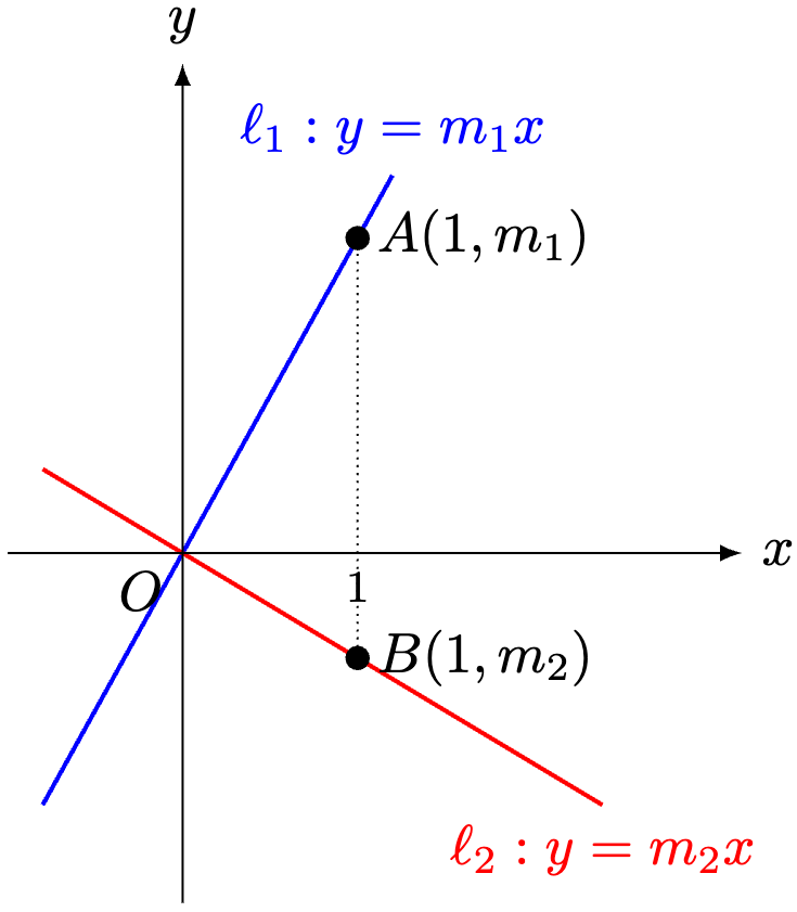
Theorem 2. Define the lines and , where . Then if and only if .
Proof Sketch. Consider the diagram below.
Using Pythagoras’ theorem,
Therefore, by Pythagoras’ theorem and its converse, if and only if :
We leave it as an exercise in algebra to simplify this equation to
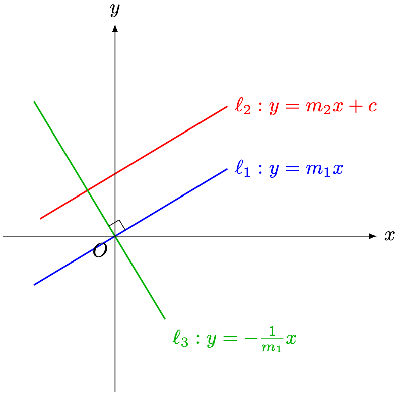
Theorem 3. Define the lines and , where . Then if and only if .
Remark 2. Observe the deliberate omission of a diagram in Theorem 3. The power of vectors (i.e. linear algebra) is to describe geometry without a need for visual representation (though the latter will be useful for us in the process of proving the result).
Proof Sketch. Define the line . By Theorem 2, since , .
Since the interior angles of a pair of lines sum to if and only if the lines are parallel,
Corollary 1. Consider the lines
where . Then if and only if .
Proof. Define . By Theorem 3, . Then by Theorem 3 again,
Theorem 4. Let be two-dimensional vectors and . Using Theorem 1, consider the lines defined by
where we abbreviate . Then if and only if there exists some real number such that .
ProofSketch. Use Theorems 1 and 3.
There are many more implications of thinking in terms of vectors, but we conclude with the famous intercept theorem.
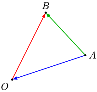
Lemma 1. Given two points , denote the vector starting at and ending at by .
Then .
Proof. Using vector addition,
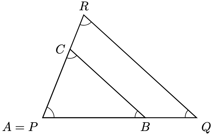
Theorem 5 (Intercept Theorem). Given three distinct points and positive numbers , define the points by and below.
(Here, we assume for simplicity.)
Then if and only if . In this case,
Proof Sketch. Denote and . By Lemma 1,
In the direction , suppose . Then
By Theorem 4, .
In the direction , Theorem 4 yields some real number such that
Now are non-zero. If , then it can be shown that , a contradiction. Therefore, we must have . Similarly, . Therefore, , in which case,
In a similar manner with the other sides,
Corollary 2 (Midpoint Theorem). If we have
then and .
Proof. By hypothesis, set in Theorem 5 to obtain , and consequently, .
In this case, we call and similar triangles, which we will revisit later on.
Using this idea of describing shapes using coordinates, we turn to parabolas, and namely, analyse graphs of the form .
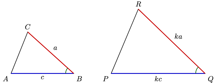
Having discussed a great deal about congruent triangles, we now turn our attention to a relaxation of congruence—similarities. Similarities are, no pun intended, similar ideas to congruence, but far more useful in helping us use small-scale items to represent large-scale items, such as maps and scale models.
Lemma 1. If , then
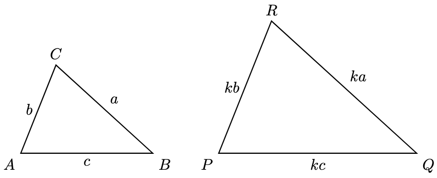
Definition 1 (SSS Similarity Definition). We say that the triangles are similar, denoted , if there exists some positive constant such that
Therefore, congruence becomes a special case of similarity via the special case .
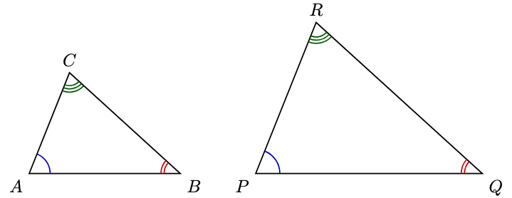
Since congruent triangles have angles that match, do similar triangles have angles match? Not only do they match, but that they have to match.
Lemma 2. We have if and only if their angles match:
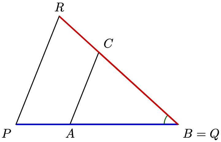
Proof Sketch. Suppose without loss of generality that . For setup, translate and rotate where necessary so that and lies on .
In the direction , suppose . Then
A technical proof by contradiction shows that must lie on . By the intercept theorem, . Using corresponding angles,
Since the angles in a triangle sum to , .
In the direction , since , must lie on . Since
using corresponding angles, . By the intercept theorem again,
yielding , as required.
Theorem 1 (AA Similarity Criterion). We have if and only if at least two of the following equalities hold:
Proof. It suffices to prove the direction . Since angles in a triangle sum to , we get all three equalities if we know at least two of them hold. By Lemma 2, the result holds.
Theorem 2 (SAS Similarity Criterion). We have if and only if
Proof Sketch. It suffices to prove the direction . Since , if lies on , then must lie on .
By the intercept theorem,
Using corresponding angles, . By the AA Similarity Criterion, .
Similar triangles are used all the time in establishing interesting result in plane geometry.
Example 1 (Tangent-Secant Theorem). In the diagram below, (this is called the alternate segment theorem).
Show that , known as the tangent-secant theorem.
Solution. Since and , by the AA Similarity Criterion, . In particular,
Example 2. In the diagram below, are distinct points that lie on a circle.
Given that is the intersection of and , show that
Solution. For the first claim, since angles in the same segment are equal (i.e. the butterfly theorem), . Since vertically opposite angles are equal, . By the AA Similarity Criterion, . In particular,
Okay, let’s return to earth one more time.
Definition 2. Denote the scale to mean that unit of length in some representation (e.g. a map, scale model, etc) represents units of length in real life.
Example 3. Suppose cm on a map represents km in real life. Determine the scale in terms of .
Solution. Since ,
Hence, the required scale is
Lemma 2. Suppose we have a scale of . Then the area scale is given by . That is, square unit of area represents square units of area in real life.
Proof Sketch. We can use the Riemann integration approach of approximating objects using a combination of squares. Since a square with length and height represents a real-life square with length and height , the real-life square has area .
Lemma 3. Suppose we have a scale of . Then the volume scale is given by . That is, cubic unit of area represents cubic units of area in real life.
Proof Sketch. Follow the idea in Lemma 2.
Likewise, using triangles to approximate shapes, two objects are similar if they share the same shape, and thus share some kind of similarity ratio in Definition 1. Therefore, the results following Definition 2 hold, allowing us to use scale models to represent real-life objects. From these ideas we obtain products like world globe maps and merchandise of varying sizes.
To further leverage these similarity properties, it helps for us to have simple formulas for well-known shapes. While we cannot prove them all in O-Level mathematics, we can state them and relegate their proofs to integral calculus. We explore these formulas in the next post.
Example 1. Given non-negative integers , show that . Furthermore, if , show that
Solution. We observe that
Since ,
For the second claim, we employ a similar strategy:
so that .
Lemma 1. is an non-negative integer if and only if there exists a non-negative integer such that , in which we write . In this case, we say that is a perfect square.
Proof Sketch. Use prime factorisation and a proof by contradiction in the spirit of proving that the number is not a fraction (i.e. an irrational number).
Lemma 2. Suppose there exist positive integers such that . Then .
Proof. By Example 1,
Example 2. Evaluate the numbers in the form , where are rational numbers.
Solution. We observe that . By Lemma 2,
Similarly, , so that by Lemma 2 again,
Lemma 3. Suppose is not a perfect square. If are rational numbers such that , then . In particular, if , then and . We call this technique comparing of coefficients.
Proof Sketch. Follow the proof strategy in Lemma 1. Left as an exercise in proof by contradiction and baby number theory for interested readers.
Definition 1. Let be a positive natural number.
We say that square-free if none of the numbers are factors of .
A real number of the form , where is square-free, is called a surd.
Given a square-free natural number , all numbers , where are rational, are real numbers. The collection of such numbers is called a quadratic field, commonly denoted .
In particular, if are integers, then is an integer as well, and the quadratic equation has roots
By Lemma 2, we still obtain two real and distinct roots. By Lemma 3, we will not be able to represent them purely using fractions.
Example 3. Evaluate in the form , where are rational numbers.
Solution. By Example 1,
By observing that ,
Therefore, .
Example 4. Given rational numbers and a non-negative integer , show that
is a rational number. Hence, evaluate in the form , where are rational numbers.
Solution. Using the difference of squares formula,
Since are rational numbers, so is .
Similar to Example 3, we observe that , so that
Remark 1. The technique in Examples 3 and 4 is called rationalising the denominator.
Example 5. Calculate the length of a square with area sqaured-units in the form , where are rational numbers.
Solution. Let denote the length of the square. Since the square has area ,
By comparing of coefficients as per Lemma 3,
Thus, we reduce the problem to solving a pair of equations, and we shall do so by substitution. Making the subject in the second equation,
Substituting this value of into the first equation,
Since is a perfect square, we could solve by either factorisation or the quadratic formula. We shall use the latter since we are lazy:
Hence, or .
In the latter case, , which is a contradiction since is a rational number and is not a rational number, therefore we reject this case, and conclude that . Hence, . Substituting into the expression for ,
Therefore, , which abbreviates the following two cases:
if , then , and
if , then .
Hence, the length of the square is either or . Since lengths are non-negative and , we reject the latter case, and conclude that the length of the square is units. In more mathematical jargon,
Example 6. Calculate the length of the base of a right-isosceles triangle with longest side length (i.e. hypotenuse) .
Solution. Denote the desired side length by . By Pythagoras’ theorem,
Taking square roots,
By rationalising the denominator,
Therefore, the triangle has base length .
Remark 2. As far as possible, we express answers involving surds in the form , where are simplified rational numbers and is square-free. In linear algebra, numbers of this form are called linear combinations of the basis.
While understanding surds of the form , where is non-negative, has its uses in simplifying otherwise complicated numerical expressions, its power becomes beefed up significantly if is negative, for example, if we consider numbers of the form .
You would scream at me for committing this mathematical crime. We have emphasised repeatedly that there is no real number such that , so how in good faith and conscience can we write and not cringe like the 6-7 kid? You are absolutely right—but we are assuming that the only numbers that we can talk about are real numbers.
Definition 1. Call the number the imaginary unit, defined by the “false” equation .
For more interested readers: legitimately defined using techniques in linear algebra here).
A number of the form , where are real numbers, is called complex.
Since , we have .
While we need a rather distinct visual idea for what means, if we allow the calculation , we recover many of the properties discussed in the previous lemmas and examples.
Theorem 1. The complex numbers satisfy the following properties:
If , then .
If are real numbers such that , then .
Given real numbers , is still a complex number.
Given real numbers , is still a complex number.
Proof Sketch. Adapt the solutions in the previous lemmas and examples.
Definition 2. Define the conjugate of a complex number by .
Example 7. Let be a complex number. Show that is a real number. Deduce that
Solution. Write , where are real numbers. Using Example 4,
which is a real number since are real numbers. In particular, if , then . Since are real numbers,
Therefore, implies that . Similarly, , so that
In particular, we can make the following claim.
Theorem 2. The solutions to the equation are given by
In particular, the solutions are
real and distinct if ,
real and repeated if ,
complex conjugates if .
Any further discussion on complex numbers is relegated to A-Level Mathematics, and so we will only explore this idea in detail when we get there.
For now, we can ask a humble yet daunting question: given real numbers where , how can we solve the cubic equation below?
We will explore this idea next time using polynomials and its cousin the partial fractions.
If the sum of angles in a -sided polygon (i.e. a -gon / tri-gon / triangle) is , what is the sum of angles in an -sided polygon (i.e. an -gon)?
Theorem 1. The sum of interior angles in an -gon is .
Proof. In the case , we have an angle sum of , as required.
In the case , the key observation is to split the -gon into a triangle and a -gon.
In Case 1, there is no reflex interior angle. In Case 2, there is at least one reflex interior angle. In either case, since the interior angle sum of a -gon is , the -gon must have an interior angle sum of
Roughly speaking, we can generalise this case using mathematical induction. Suppose that a -gon has interior angle sum of . Then we can split the -gon into a triangle and a -gon. Since the triangle has interior angle sum of and the -gon has interior angle sum of , the -gon has interior angle sum of
Therefore, if the result holds for , it holds for , and subsequently, , and so on and so forth. Therefore, any -gon must have an interior angle sum of .
Definition 1. An -sided polygon is convex if it does not have any reflex interior angle.
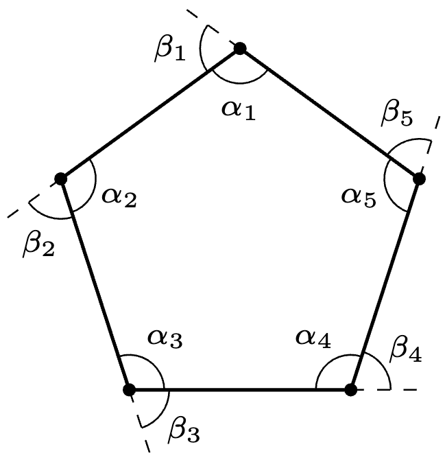
Theorem 2. The sum of exterior angles for any convex -gon is .
Proof. Recall that the exterior angle is the angle that lies on the same straight line as the interior angle that it is adjacent to (the diagram shows the case of a -gon, and there’s no requirement that the polygon be regular).
Let denote the -th interior and exterior angle respectively. Since adjacent non-overlapping angles on a straight line sum to ,
Adding all pairs of angles together,
By Theorem 1,
Therefore, substituting into the original equation,
Definition 2. A polygon is regular if all of its interior angles are equal.
Corollary 1. The interior angle of a regular -gon is .
What about circles? Circles have an interesting cousin that we will care about a lot. Recall that a circle is a set of points that are located a fixed distance , called the radius, away some fixed centre point.
Definition 3. Let be a point and be a point not on . A parabola with focus and directrix is the set of points whose distance to and are equal.
Theorem 3. Fix . The equation of a parabola with focus and directrix is given by . In particular, it contains the point .
Proof. Let be any point on the parabola. Using Pythagoras’ theorem,
By definition of the distance to a line, its distance from is given by . By the definition of a parabola,
Remark 1. Defining , we get the equation . Since it must pass through the points and , decreases as increases, so that the resulting parabola becomes steeper.
Theorem 4. Let , be constants. Then the quadratic graph with equation will always be a parabola with some focus and horizontal directrix , where are constants in terms of .
Proof. We claim that there exists real constants in terms of such that
In this case, we can define and obtain a focus of and a directrix with equation .
To make our case, expand the right-hand side:
Therefore, ensure and by setting
If we expand the right-hand side of , we get
where the quantity is called the discriminant of the quadratic function. Finally, we have as the turning point of the parabola.
Remark 1. The derivation of is known as completing the square on the right-hand side.
Corollary 2. The graph of lies on a parabola with focus and directrix .
Proof. By considering the equation , we set in Theorem 4 to obtain , so that we recover a focus of and directrix of . Now replace with to obtain the desired result.
The cousins of the circle and the parabola would be the ellipse and hyperbola respectively, and together, these shapes constitute the four famous conic sections. Deriving their equations follows in spirit with the parabola, albeit requiring a little more tedious bookkeeping. Perhaps these graphs are better left as an exercise.
Before we proceed to the next large sub-topic in secondary school mathematics, namely algebra, it might help us to explore its bridge, linear algebra, with a little more detail. The main object of interest would be the vector, and vectors turn out to help us conceptualise many geometric ideas using coordinates and algebraic calculations.
Recall that a circle with centre and radius is simply the set of points whose distance from is .
This circular equidistant property is the vital source of many seemingly magical circle properties—and the isosceles triangle will help us greatly in this task.
Definition 1. For any two distinct points on a circle, we call a chord, and the regions that it divides the circle into its segments.
The segment with smaller area is called the minor segment, and the segment with larger area is called the major segment.
Theorem 1. Let be points on a circle with centre . We call the angle subtended by the chord .
Then . That is, the angle at the centre of the circle equals two times the corresponding angle at its circumference. By “corresponding” we mean that lie in the same segment.
Proof. Connect as follows and extend to the opposite end of the circle (i.e. turn it into a diameter).
Observe that as radii (plural for radius) of the same circle, . Hence, the triangles and are isosceles, and their respective base angles equal each other:
Since the external angle of the triangle equals the sum of the corresponding opposite interior angles,
Similarly, . Therefore,
Remark 1. If is obtuse, then the argument still holds and . In this case, we say that is reflex.
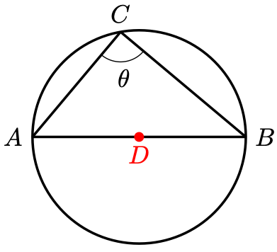
Corollary 1 (Thale’s Theorem). Consider the points on the circle below.
Then if and only if is a diameter of the circle.
Proof. Denote the centre of the circle by .
By Theorem 1,. Hence,
which holds if and only if lies on , and that holds if and only if is a diameter.
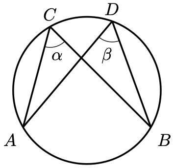
Corollary 2. Consider the points on the circle below.
Then . That is, angles subtended by the same chord equal each other.
Proof. Denote the centre of the circle by .
Applying Theorem 1 twice,
Therefore, .
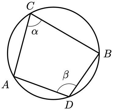
Corollary 3. Consider the points on the circle below.
Then . That is, angles in opposite segments sum to (i.e. are supplementary).
Proof. Denote the centre of the circle by .
By Theorem 1, . By Theorem 1 again, the reflex angle of equals . Since angles at a point sum to ,
While we have derived many useful angle properties pertaining circles, the chords themselves are worth just as much attention, and their proofs aren’t even too difficult!
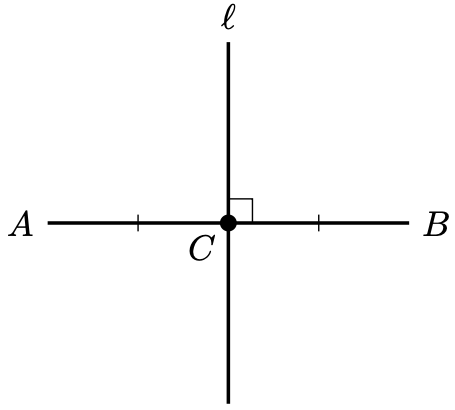
Definition 2. The midpoint of a line segment is the point such that .
Call the line the perpendicularbisector of if and it intersects at the midpoint of .
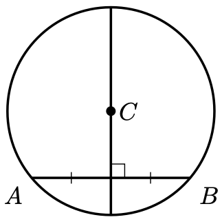
Theorem 2. Consider the points on the circle with centre below.
Then the perpendicular bisector of will always intersect .
Proof. Construct the edges and for visibility and construct the altitude from to .
Since are radii of the same circle, . Since adjacent angles on a straight line are supplmenetary, . Since is a common side, by the RHS Criterion, .
In particular, , which means that lies on the perpendicular bisector of . Therefore, lies on the perpendicular bisector of , as required.
Definition 3. Define the distance from a point to a line to be the shortest distance between the point and any point on the line.
By Pythagoras’ theorem, this distance must be the length of the altitude from , perpendicular to .
Theorem 3. Consider the points on the circle with centre below.
Then if and only if .
Proof. Construct the edges for visibility.
Since are radii of the same circle, . By various triangle congruence criteria (left as an exercise),
There are several more properties needed to properly conclude our discussion on circles, but we will relegate them as exercises in proving techniques.
For now, we need to consider other kinds of shapes, such as four-sided shapes, known as quadrilaterals, as well as more general -sided shapes called polygons. We don’t need any new machinery—all that we have discussed so far is enough to establish these results, which we will explore next time.


 (units) long and height
  .
.
 as real numbers.
 .
.
 ,
,

 . Consider the new triangle with area
  as follows:
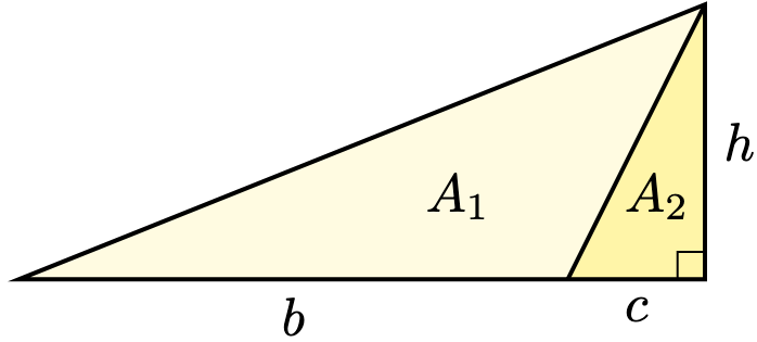


 and height
  .
.

 .
. , by Theorem 2, its area is given by
 , but how do we get that formula in the first place?
 and radius
  to be the constant
 . Numerically,
  .
.
 sub-divisions for convenience. We notice that the areas total to the circle area. By rearranging these sectors, we recover an approximate rectangle with approximate base
  and approximate height
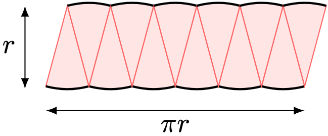
 . Increasing the number of subdivisions improves the approximation, and in the limit, we get an exact area of
  (i.e.
(i.e.  degrees) to denote the angle of a “complete turn”. The reason for
  that find many uses in astronomy and geology. In particular,
  denotes a
  -turn,
  denotes a
  -turn, so on and so forth.
 , then its circumference is
  :
:
 denotes a complete turn. In particular,
  . In this case, we say that the angle is
  radians if the corresponding curved segment (i.e. arc) in the unit circle has a length of
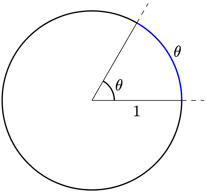
 is given by
 . In particular,
  , agreeing with our prior intuitions on the circumference.
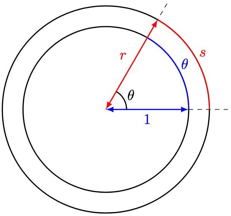


 .
. . In particular, with a full circle, we obtain the expected area
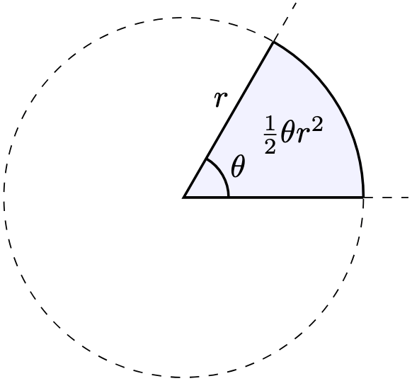
 of the original circle, its area would correspond to
 to obtain an area of
  .
. :
:
 :
:
 , and even binomials such as
  . Much of our exploration arises from interpreting powers as repeated multiplication in the following sense: given any positive number
  and positive integers
  ,
,
 , for real numbers
 the base–
 .
.![\displaystyle a^0 = 1, \quad a^{1/n} = \sqrt[n]{a}, \quad a^{-x} = \frac 1{a^x}, \quad a^{x-y} = \frac{ a^x }{ a^y }.](https://s0.wp.com/latex.php?latex=%5Cdisplaystyle+a%5E0+%3D+1%2C+%5Cquad+a%5E%7B1%2Fn%7D+%3D+%5Csqrt%5Bn%5D%7Ba%7D%2C+%5Cquad+a%5E%7B-x%7D+%3D+%5Cfrac+1%7Ba%5Ex%7D%2C+%5Cquad+a%5E%7Bx-y%7D+%3D+%5Cfrac%7B+a%5Ex+%7D%7B+a%5Ey+%7D.&bg=ffffff&fg=000&s=0&c=20201002)
 refers to a positive integer, and
  refers to real numbers.
 ,
,
![(a^{1/n})^n = \underbrace{a^{1/n} \cdot a^{1/n} \cdot \cdots \cdot a^{1/n}}_n = a^{n \cdot (1/n)} = a\quad \Rightarrow \quad \boxed{ a^{1/n} = \sqrt[n]{a} }.](https://s0.wp.com/latex.php?latex=%28a%5E%7B1%2Fn%7D%29%5En+%3D+%5Cunderbrace%7Ba%5E%7B1%2Fn%7D+%5Ccdot+a%5E%7B1%2Fn%7D+%5Ccdot+%5Ccdots+%5Ccdot+a%5E%7B1%2Fn%7D%7D_n+%3D+a%5E%7Bn+%5Ccdot+%281%2Fn%29%7D+%3D+a%5Cquad+%5CRightarrow+%5Cquad+%5Cboxed%7B+a%5E%7B1%2Fn%7D+%3D+%5Csqrt%5Bn%5D%7Ba%7D+%7D.&bg=ffffff&fg=000&s=0&c=20201002)


 (it is
  ), we would also like to solve equations such as
  . We observe that, rather straightforwardly, if
  is an integer, then
 logarithm of
  with
with 
 .
.

 . By Definition 1,
 .
. , we have the following laws of logarithms:
 , and for any
  ,.
,.

 . For the last property, we prove the special case that


 , demonstrate the existence of irrational numbers
  such that
  is rational. You may assume without proof that
  is irrational.
 yields
 and
and  yields, by Corollary 1,
 ,
,
 and
and  , where

 logarithm finds much use in numerically estimating the logarithms. For instance, the pH of a solution that measures the acidity of that solution (crucial in ecological applications) is defined by the number
 ![-\lg([\mathrm H^+])](https://s0.wp.com/latex.php?latex=-%5Clg%28%5B%5Cmathrm+H%5E%2B%5D%29&bg=ffffff&fg=000&s=0&c=20201002) , where
, where ![[\mathrm H^+]](https://s0.wp.com/latex.php?latex=%5B%5Cmathrm+H%5E%2B%5D&bg=ffffff&fg=000&s=0&c=20201002) denotes the concentration of protons in that solution. The base-
denotes the concentration of protons in that solution. The base- logarithm finds much use in theoretical analysis, since the rate of change of the function
  is
is  .
. looks like the diagram below.
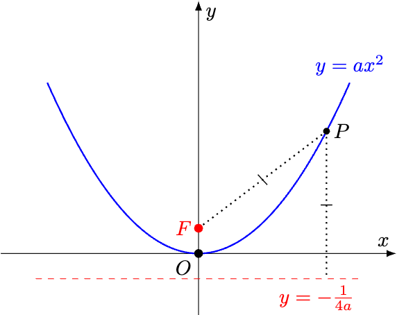
 on the graph, it has the same distance to the (focal) point
  and the (directrix) line
  . Hence, its shape is known as a parabola. In particular, it has a minimum point
  .
. .
.
 , then the whole graph gets “flipped” to the downside:
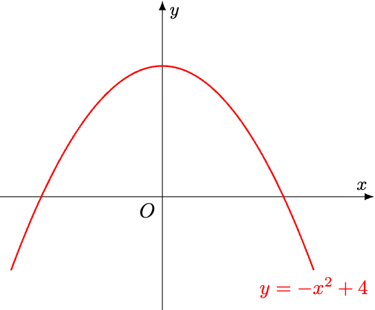
 .
. -intercept of the quadratic graph
  . Since the
 . No surprises there.
  . Since the
 so that our
  . However, this solution is only partially correct. Just like any solution in Singapore or US politics.
 , we must conclude either possibility, namely, that
  or
or  . To abbreviate, we use the
  notation:
  . This notation states that either
  or
or  are plausible values that
  and
and  .
.
 , where
  respectively.
 . Therefore,

 , then
  . Taking square roots,
 or
or  , yielding the
  and
and  .
. , then
  . Taking square roots,
 or
or  , yielding the
  and
and  .
. , then
  . Taking square roots,
 , yielding only one
  .
. , then
  . Now, if
  is a real number too, which implies that
  . Therefore,
  . This can only mean that the equation
  has no real solutions, and therefore, the graph of
  no
no 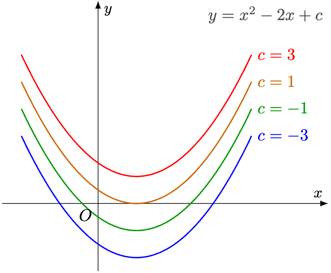
 , and determine them in terms of
 ,
,  , or
, or  .
.
 , so that
  . Hence,
 and
and  .
.
 .
. , so that
 has no real solutions, and the graph has no
  is called the line of symmetry of the graph, and the point
  is a real number solution of the quadratic equation
  if
if  . Equivalently,
 ,
, is an
is an 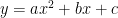 .
. . Define the discriminant
  of the quadratic equation by
 ,
, , and
, and real number solutions if
  .
. are given by the quadratic formula:
 in terms of
  such that

 ,
,
 has the roots given by
  . We will explore expressions of this form in the next post.
 with
with  a cubic graph.
 .
. , so that
 . Repeat the procedure to deduce that
  as well.
 , where
 a polynomial function, properly defined using
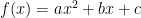
 is called a linear function, since
  grows linearly in the following sense:
 is called a constant function, since no matter what input number
  ,
,  is a factor of
  .
. , we use the difference of squares property:
 is a factor of
  . For the case
  , we seek constants
  such that

 , we must stipulate
  and
and

 .
.
 such that
 is a
is a  .
. and a unique real number
 . Furthermore,
 , which holds if and only if
  has one solution given by
  . We first observe that


 and
and 
 . Therefore,

 or
or  . In the former,
 .
. such that equation
 . Using the
  is a factor of
  .
. is a solution of the equation
  . By the factor theorem,
  is a factor of
  . Hence, there exist real constants
 , so that
 , we use the quadratic formula:
 .
. , we can show that
 a cyclic group under multiplication, and thus Abelian, since

 ? We explore the answer to this question when discussing the binomial theorem.
 .
. for some positive number
  , we have the following more refined definition of a magnitude.
 the absolute value of
  ; indeed, the number
  , visualised using a two-dimensional arrow in the
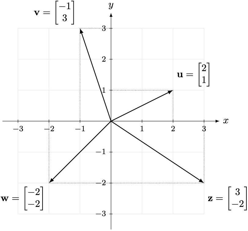


 .
.
 , then
  .
. , then
  and
and  .
. . Therefore,
 and
and  below.
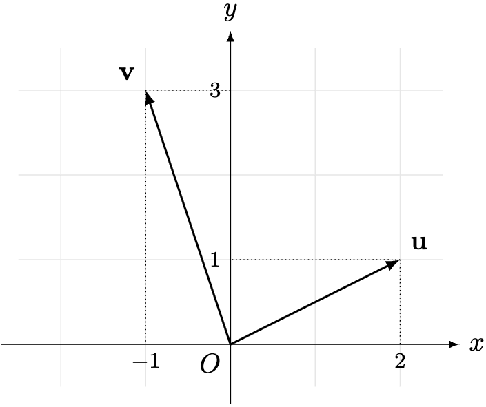
 ? Intuitively, it means that starting from the point
  , then continue our journey according to
  . This process is equivalent to sliding the ‘tail’ of
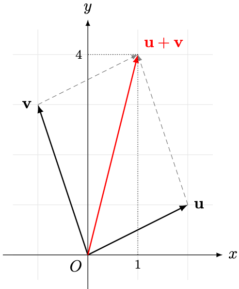


 , define:
 , and
, and .
. . Evaluate separately the quantities
  ,
,  , and
, and  .
. . By the definition of vector addition,


 . Then there exist two-dimensional vectors
  such that
 the direction vector of
  and
and  , and verify that the equation holds.
 and
and  , where
  . Then
  if and only if
  .
.

 if and only if
  :
:

 , where
  . Then
  if and only if
  .
. . By Theorem 2, since
  ,
,  .
.
 if and only if the lines are parallel,

 . By Theorem 3,
  . Then by Theorem 3 again,
 be two-dimensional vectors and
  . Using Theorem 1, consider the lines
  defined by
 . Then
  .
. , denote the vector starting at
  by
by  .
.
 .
.
 and positive numbers
  , define the points
  by
by  and
and  below.
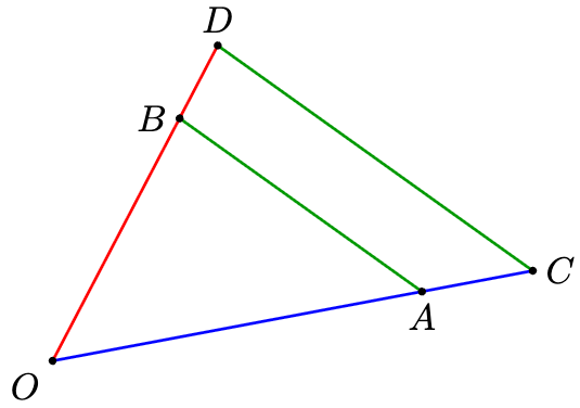
 for simplicity.)
 if and only if
  . In this case,
 and
and  . By Lemma 1,
 , suppose
  . Then
 , Theorem 4 yields some real number
 are non-zero. If
  , then it can be shown that
  , a contradiction. Therefore, we must have
  . Similarly,
  . Therefore,
  , in which case,


 .
. in Theorem 5 to obtain
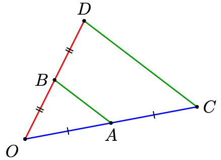
 and
and  similar triangles, which we will revisit later on.
 , then
 are similar, denoted
  , if there exists some positive constant
 .
.

 . For setup, translate and rotate
  where necessary so that
  and
and  .
.

 . By the intercept theorem,
  . Using corresponding angles,
 .
.


 , if
, if  .
.

 (this is called the alternate segment theorem).
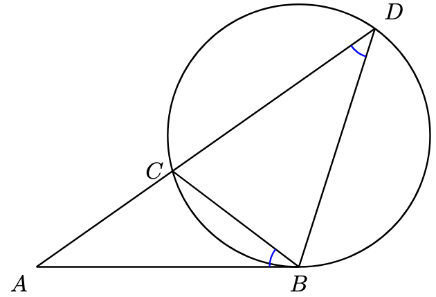
 , known as the tangent-secant theorem.
 and
and  , by the AA Similarity Criterion,
  . In particular,
 are distinct points that lie on a circle.
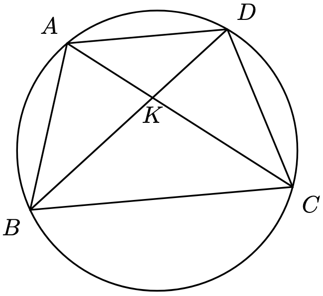
 is the intersection of
  and
and  , show that
 . Since vertically opposite angles are equal,
  . By the AA Similarity Criterion,
  . In particular,
 to mean that
  units of length in real life.
 km in real life. Determine the scale in terms of
  ,
,

 . That is,
  square units of area in real life.
 .
. . That is,
  cubic units of area in real life.

 is a unique
  . Furthermore, if
  , show that

 ,
,

 .
. , in which we write
  . In this case, we say that
  such that
  . Then
  .
.
 in the form
  , where
  . By Lemma 2,
 , so that by Lemma 2 again,
 , then
  , then
  and
and  . We call this technique comparing of coefficients.
 are factors of
  , where
  , where
  .
. are integers, then
  is an integer as well, and the quadratic equation has roots
 in the form
  , where
 ,
,
 .
.
 in the form
 are rational numbers, so is
  .
. , so that
 sqaured-units in the form
  denote the length of the square. Since the square has area


 is a perfect square, we could solve by either factorisation or the quadratic formula. We shall use the latter since we are lazy:
 or
or  .
. , which is a contradiction since
  . Substituting into the expression for
 , which abbreviates the following two cases:
 , then
  , and
, and , then
  .
. or
or  . Since lengths are non-negative and
  , we reject the latter case, and conclude that the length of the square is
  units. In more mathematical jargon,


 .
. , where
  .
. .
. , so how in good faith and conscience can we write
  the imaginary unit, defined by the “false” equation
  .
. , where
  , we have
  .
. .
. , then
  .
. is still a complex number.
 is still a complex number.
 .
. be a complex number. Show that
  is a real number. Deduce that
 , where
 , then
  . Since
 implies that
  . Similarly,
  , so that
 .
. , as required.
 , the key observation is to split the
  -gon into a triangle and a
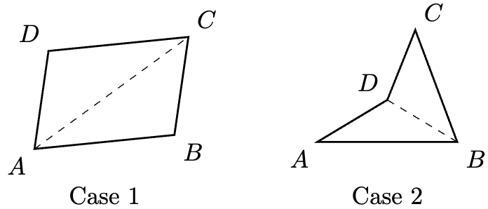

 . Then we can split the
  -gon into a triangle and a
 , it holds for
  , and subsequently,
  , and so on and so forth. Therefore, any
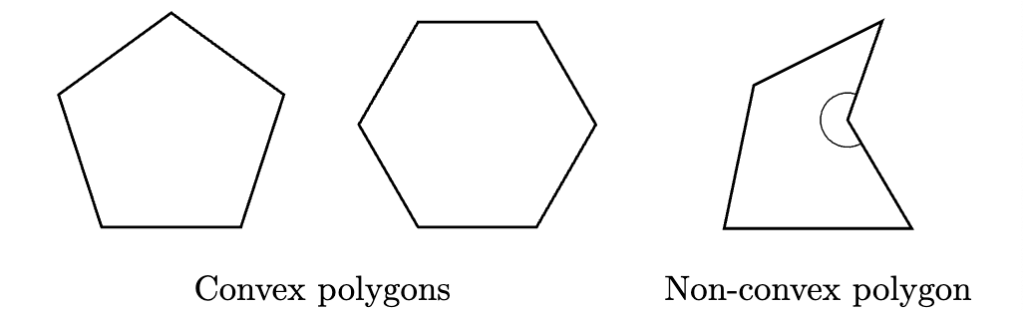
 denote the


 .
. be a point not on
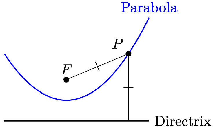
 . The equation of a parabola with focus
  and directrix
  is given by
  . In particular, it contains the point
  be any point on the parabola. Using Pythagoras’ theorem,
 . By the definition of a parabola,
 , we get the equation
  ,
,  decreases as
  be constants. Then the quadratic graph with equation
  and horizontal directrix
  , where
  are constants in terms of
 and obtain a focus of
  .
.
 and
and  by setting

 is called the discriminant of the quadratic function
  lies on a parabola with focus
  and directrix
  .
.
 , we set
  in Theorem 4 to obtain
  , so that we recover a focus of
  and directrix of
  . Now replace
  with
with  to obtain the desired result.
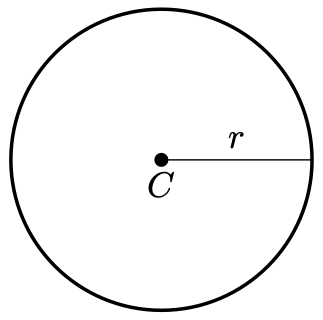
 on a circle, we call
  a chord, and the regions that it divides the circle into its segments.
 be points on a circle with centre
  the angle subtended by the chord
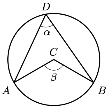
 . That is, the angle at the centre of the circle equals two times the corresponding angle at its circumference. By “corresponding” we mean that
  lie in the same segment.
 as follows and extend
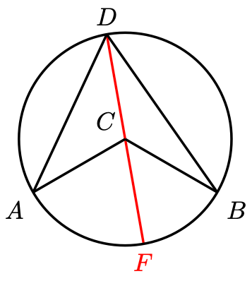
 . Hence, the triangles
  and
and  are isosceles, and their respective base angles equal each other:
 equals the sum of the corresponding opposite interior angles,
 . Therefore,
 is obtuse, then the argument still holds and
  . In this case, we say that
  is reflex.
 on the circle below.
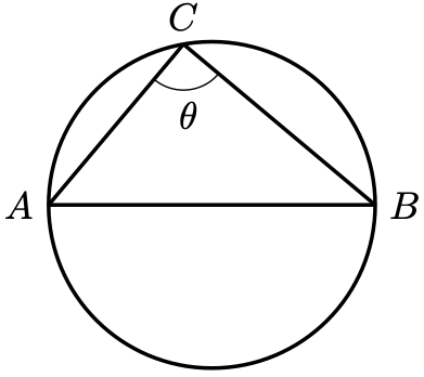
 if and only if
  .
.
 . Hence,
 . That is, angles subtended by the same chord equal each other.
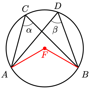

 .
.
 . That is, angles in opposite segments sum to
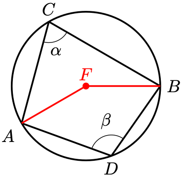
 . By Theorem 1 again, the reflex angle of
  equals
  . Since angles at a point sum to
 .
.
 and it intersects
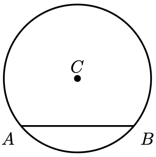
 for visibility and construct the altitude from
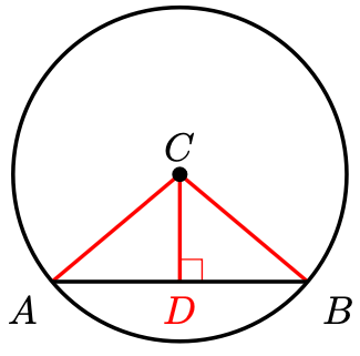
 are radii of the same circle,
  . Since adjacent angles on a straight line are supplmenetary,
  . Since
  .
. , which means that
  to a line
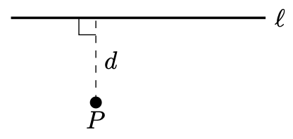
 on the circle with centre
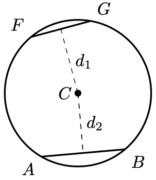
 if and only if
  .
. for visibility.
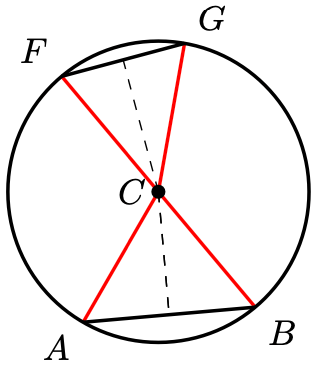
 . By various triangle congruence criteria (left as an exercise),

_without_New_Guinea.svg)