Skip to content

KindiakMath

About
- Curriculum Vitae
- Review Quotes
Pre-University
Foundational Math
Theoretical Analysis
Unified Math
- Complex Analysis
- Abstract Algebra
Para-Mathematics

Category: Probability

Jordan Decomposition
This post is inspired by Professor Tom Fischer’s writeup.

Recall the Hahn decomposition theorem:

Theorem 1. If $\mu$ is a signed measure on $(\Omega, \mathcal F)$ , then there exist disjoint measurable subsets $P, N \in \mathcal F$ such that

$\mu (\cdot \cap P) \in [0, \infty),\quad \mu (\cdot \cap N) \in (-\infty, 0] ,\quad P \sqcup N = \Omega.$

We call $P$ a positive set, denoted $P \geq 0$ , and $N$ a negative set, denoted $N \leq 0$ , and we call the pair $(P, Q)$ a Hahn decomposition for $\mu$ .

Call a set $M$ is $\mu$ –null if it is positive and negative: $\mu( \cdot \cap M) \in \{0\}$ .

Define the symmetric difference by

$K\triangle L := (K \backslash L) \sqcup (L \backslash K).$

We leave it as an exercise to verify that

$K \cup L = (K \cap L) \sqcup (K\triangle L).$

Problem 1. Let $\mu$ be a signed measure on $(\Omega, \mathcal F)$ and $(P_1,N_1)$ , $(P_2,N_2)$ be two Hahn decompositions for $\mu$ . Show that $P_1 \triangle P_2$ and $N_1 \triangle N_2$ are $\mu$ -null.

(Click for Solution)

Solution. Fix $K \in \mathcal F$ . Then

$\begin{aligned} \mu(K \cap (P_1 \triangle P_2)) &= \mu(K \cap P_1 \backslash P_2) + \mu(K \cap P_2 \backslash P_1) \\ &= \mu(K \cap P_1 \cap N_2) + \mu(K \cap P_2 \cap N_2) \\ &= \mu(K \cap P_1 \cap N_2) + \mu(\emptyset) \\ &= \mu(K \cap P_1 \cap N_2). \end{aligned}$

Using Theorem 1,

$\begin{aligned} 0 &\leq \mu((K \cap N_2) \cap P_1) \\ &= \mu(K \cap P_1 \cap N_2) \\ &= \mu((K \cap P_1) \cap N_2) \leq 0, \end{aligned}$

so $\mu(K \cap (P_1 \triangle P_2)) = \mu(K \cap P_1 \cap N_2) = 0$ , as required.

We now state the Jordan decomposition theorem.

Problem 2. Let $\mu$ be a finite signed measure on $(\Omega, \mathcal F)$ . Construct unique finite measures $\mu^+, \mu^-$ on $(\Omega , \mathcal F)$ such that:
- $\mu = \mu^+ - \mu^-$ , and
- for any Hahn decomposition $(P, N)$ of $(\Omega, \mathcal F)$ , $\mu^+(K) = 0$ for $K \subseteq N$ and $\mu^-(K) = 0$ for $K \subseteq P$ .
We call $(\mu^+, \mu^-)$ the (unique) Jordan decomposition of $\mu$ .

(Click for Solution)

Solution. Use Theorem 1 to construct a Hahn decomposition $(P_1, N_1)$ . Define

$\begin{aligned} \mu^+ &:= \mu(\cdot \cap P_1) \in [0, \infty),\\ \mu^- &:= -\mu(\cdot \cap N_1) \in [0, \infty). \end{aligned}$

Then for any $K \in \mathcal F$ ,

$\begin{aligned} \mu(K) &= \mu(K \cap P_1) + \mu(K \cap N_1) \\ &= \mu^+(K) - \mu^-(K) \\ &= (\mu^+ - \mu^-)(K). \end{aligned}$

Hence, $\mu = \mu^+ - \mu^-$ .

Now fix any Hahn decomposition $(P_2, N_2)$ . Then

$\begin{aligned} P_1 &= P_1 \cap (P_1 \cup P_2) \\ &= P_1 \cap ((P_1 \cap P_2) \sqcup (P_1 \triangle P_2)) \\ &= (P_1 \cap (P_1 \cap P_2)) \sqcup (P_1 \cap (P_1 \triangle P_2)) \\ &= (P_1 \cap P_2) \sqcup (P_1 \cap (P_1 \triangle P_2)).\end{aligned}$

Fix $K \subseteq N_2$ . Then

$\begin{aligned} \mu^+(K) &= \mu(K \cap P_1) \\ &= \mu(K \cap P_1 \cap P_2) + \mu(K \cap P_1 \cap (P_1 \triangle P_2)) \\ &= \mu(K \cap \emptyset) + \mu((K \cap P_1) \cap (P_1 \triangle P_2)) \\ &= 0 + 0 = 0. \end{aligned}$

Similarly, $K \subseteq P_2$ implies $\mu^-(K) = 0$ .

Finally, we establish the uniqueness of the measures. Suppose

$\mu = \mu_1^+ - \mu_1^- = \mu_2^+ - \mu_2^-.$

We need to check that $\mu_1^+ = \mu_2^+$ . To that end, fix any Hahn decomposition $(P, N)$ . For any $K \subseteq P$ ,

$\mu_1^+(K \cap N) = 0 = \mu_2^+(K \cap N)$

and

$\mu_1^-(K) = 0 = \mu_2^-(K)$

so that

$\begin{aligned} \mu_1^+(K) &= \mu(P) - \mu_1^-(K) \\ &= \mu(P) - \mu_2^-(K) = \mu_2^+(K). \end{aligned}$

Hence, for any $K = (K \cap P) \sqcup (K \cap N)$ ,

$\begin{aligned} \mu_1^+(K) &= \mu_1^+(K \cap P) + \mu_1^+(K \cap N) \\ &= \mu_2^+(K \cap P) + \mu_2^+(K \cap N) = \mu_2^+(K). \end{aligned}$

—Joel Kindiak, 7 Jan 26, 1212H
March 30, 2026
Risky Bernoulli Bandits
In this appendix for the multi-armed bandit writeups, I thought I’d revisit my final year project in a relatively readable manner, demonstrating how $\rho$ -Thomoson Sampling is asymptotically optimal for Bernoulli bandits (that is, $\nu_i = \mathrm{Ber}(p_i)$ for each $i$ ). This is the instantiation $M = 1$ of my final year project.

As a set-up, we initialise $\mathbb P_{i,0} = \mathrm{Beta}(\alpha, \beta)$ with p.d.f.

$\displaystyle f_{\alpha , \beta}(x) = \frac{\Gamma(\alpha + \beta)}{\Gamma(\alpha) \Gamma(\beta)} \cdot x^{\alpha - 1} \cdot (1-x)^{\beta - 1},$

since the conjugate prior of a Bernoulli distribution is the Beta distribution. For the update function, we use

$\mathrm{Update}(\Gamma(\alpha, \beta)) = \Gamma(\alpha+ 1,\beta)$

and $\mathbb P_{i,t+1} = \mathrm{Update}(\mathbb P_{i,t})$ . At each time $t$ , we sample $\theta_{i,t+1} \sim \mathbb P_{i,t}$ and pull the arm

$\displaystyle A_{t+1} = \underset{i=1,\dots, K}{\arg \max}\ \rho(\mathrm{Ber}( \theta_{i,t+1} )).$

Observe that the map $p \mapsto \mathrm{Ber}(p) \mapsto \rho(\mathrm{Ber}(p))$ induces a unique map $\tilde{\rho} : [0, 1] \to \mathbb R$ given by $\tilde{\rho} = \rho(\mathrm{Ber}(p))$ . Following the Thompson sampling strategy, we need to obtain useful tail concentration bounds. We will impose some technical conditions on the risk functional $\rho$ to make this happen.

Definition 1. Call a risk functional $\rho$ continuous if $\tilde{\rho} : [0,1] \to \mathbb R$ is continuous.

If $\rho$ is continuous, then by the extreme value theorem, $\tilde{\rho}([0,1])$ is compact. Hence, there exists $p_1, p_2 \in [0,1]$ such that for any $p \in [0, 1]$ ,

$\tilde{\rho}(p_1) \leq \tilde{\rho}(p) \leq \tilde{\rho}(p_2).$

Lemma 1. If $\rho$ is continuous, then for any $p \in [0,1]$ and $r \in \mathbb R$ , there exists $p_* \in [0, 1]$ such that

$\mathcal{K}_{\inf}^{\rho}(\mathrm{Ber}(p), r) \equiv \mathcal{K}_{\inf}^{\rho}(\mathrm{Ber}(p), r, \mathrm{Ber}) = \mathrm{KL}(\mathrm{Ber}(p), \mathrm{Ber}(p_*)).$

Proof. By definition,

$\displaystyle \mathcal{K}_{\inf}^{\rho}(\mathrm{Ber}(p), r, \mathrm{Ber}) = \inf_{q : \tilde{\rho}(q) > r} \underbrace{ \mathrm{KL}(\mathrm{Ber}(p), \mathrm{Ber}(q)) }_{f(q)}.$

By a direct computation,

$\displaystyle \mathcal{K}_{\inf}^{\rho}(\mathrm{Ber}(p), r, \mathrm{Ber}) = \inf_{q : \tilde{\rho}(q) > r} \underbrace{ p \log \frac pq + (1-p) \log \frac{1-p}{1-q} }_{f(q)},$

so that $f$ is continuous on $(0, 1)$ .

If $r < \tilde{\rho}(p_1)$ , then we may simply choose $p_* = p$ . If $r \geq \tilde{\rho}(p_2)$ , then the constraint set is empty and the left-hand side is infinite, so we choose $p_* = 0$ if $p \neq 0$ and $p_* = 1$ otherwise.

Suppose $\tilde{\rho}(p_1) \leq r < \tilde{\rho}(p_2)$ . If $p = 0$ or $p = 1$ , then $f(q) = 0$ identically, so that we can choose $p_* = p_2$ .

Suppose instead that $p \in (0, 1)$ . Fix $\epsilon \in (0, \tilde{\rho}(p_2) - r)$ . Then $[r + \epsilon, \tilde{\rho}(p_2)]$ is compact, so that

$\tilde{\rho}^{-1}( [r + \epsilon, \infty) ) = \tilde{\rho}^{-1}( [r+ \epsilon, \tilde{\rho}(p_2) ] )$

is closed and bounded, and thus compact by the Heine-Borel theorem. Since the sets

$\begin{aligned} C_1(\epsilon) &:= \tilde{\rho}^{-1}( [r+ \epsilon, \infty) ) \cap [0, p],\\ C_2 (\epsilon)&:= \tilde{\rho}^{-1}( [r+ \epsilon, \infty) ) \cap [p, 1], \end{aligned}$

are also compact, we can define their extrema

$q_1(\epsilon) := \max C_1(\epsilon), \quad q_2(\epsilon) := \min C_2(\epsilon).$

At least one of these sets will always be non-empty, since $r_2 \in [0, 1]$ and $\rho(r_2) > r+\epsilon > r$ . If $C_1(\epsilon)$ is always empty, then we can omit its discussion later on. However, if $C_1(\epsilon_0) \neq \emptyset$ for some $\epsilon_0$ , then $C_1(\epsilon) \neq \emptyset$ for any $\epsilon \in (0, \epsilon_0)$ . Without loss of generality then, we assume both sets are non-empty for some sufficiently small $\epsilon > 0$ .

Using monotonicity properties, $f(q_j(\epsilon)) \leq f(q)$ for any $q \in C_j(\epsilon)$ . Therefore,

$\displaystyle \inf_{q \in C_j(\epsilon)} f(q) = f(q_j(\epsilon)).$

Now it is clear that $C_j(\epsilon_1) \subseteq C_j(\epsilon_2)$ whenever $\epsilon_1 \geq \epsilon_2$ . By the monotone convergence theorem, there exist $q_j \in [0,1]$ such that $q_j(1/n) \to q_j$ and

$\displaystyle \inf_{q \in C_j(0)} f(q) = f(q_j).$

Define $C_j'(\epsilon) := C_j(\epsilon) \backslash \rho^{-1}(r)$ . Since smaller sets yield larger infimums, for sufficiently large $n$ ,

$\displaystyle f(q_j) = \inf_{q \in C_j(0)} f(q) \leq \inf_{q \in C_j'(0)} f(q) \leq \inf_{C_j(1/n)} f(q) \leq f(q_j(1/n)).$

Taking $n \to \infty$ , by the squeeze theorem,

$\displaystyle \inf_{q \in C_j'(0)} f(q) = f(q_j).$

Finally, choose

$\displaystyle p_* = \underset{j=1,2}{\arg \min}\ f(q_j),$

to deduce that

$\mathcal{K}_{\inf}^{\rho}(\mathrm{Ber}(p), r, \mathrm{Ber}) = f(p_*) = \mathrm{KL}(\mathrm{Ber}(p), \mathrm{Ber}(p_*)).$

Remark 1. Most arguments in Lemma 1 boils down to the compactness of $[a, b]$ , and by extension, the space $\mathrm{Ber}$ of Bernoulli distributions, as well as the relative continuity properties of $\tilde{\rho}$ and $\mathrm{KL}(\cdot, \cdot)$ . Here are some proposed steps for further exploration:
- Generalise the risk functional to $\rho : \mathcal C \to \mathbb R$ , where $\mathcal C$ is a space of probability distributions that is compact under a suitable metric or topology.
- We would probably need to partition $\mathcal P = \{M_1,\dots, M_n\}$ into $n$ compact sets, then define the compact sets $C_n(\epsilon) = \tilde{\rho}^{-1}([r+\epsilon, \infty)) \cap M_n$ .
- During the sequential argument, we could use sequential compactness to concoct a convergent subsequence $q_j(1/n) \to q$ in place of a by-default convergent subsequence. That way, we might still be able to infimise over $C_j(0)$ via $C_j(1/n)$ .
- Since we only care about infimising, we do not need the strength of full continuity for $\mathrm{KL}(\cdot,\cdot)$ ; rather we would only require its lower semi-continuity property, which could be conceived as the “lower half” of vanilla continuity.
Thanks to the continuity of $\rho$ , we can obtain the pleasant tail upper bounds below.

Theorem 1. Fix $r \in \mathbb R$ and natural numbers $\alpha, \beta$ , $n := \alpha + \beta$ . Then there exists a universal constant $C_1$ such that for any random variable with Beta distribution $X \sim \mathrm{Beta}(\alpha, \beta)$ ,

$\begin{aligned} \mathbb P(\tilde{\rho}(X) \geq r) &\leq C_1\sqrt{n} \cdot \exp( -n \cdot \mathcal{K}_{\inf}^{\rho}(\mathrm{Ber}(\alpha/n), r) ), \\ \mathbb P(\tilde{\rho}(X) \leq r) &\leq C_1\sqrt{n} \cdot \exp( -n \cdot \mathcal{K}_{\inf}^{\rho}(\mathrm{Ber}(\alpha/n), r) ). \end{aligned}$

Proof. Denote the closed (and thus, compact) sets $S_1 := \tilde{\rho}^{-1}([r,\infty))$ and $S_2 := \tilde{\rho}^{-1}((-\infty, r])$ . Use Lemma 1 to construct $p_* \in [0, 1]$ such that

$\mathcal{K}_{\inf}^{\rho}(\mathrm{Ber}(\alpha/n), r) ) = \mathrm{KL}(\mathrm{Ber}(\alpha/n), \mathrm{Ber}(p_*)) \equiv \mathrm{KL}(\alpha/n, p_*)$

for brevity. Using the conjugate-prior connection between Beta distributions and Bernoulli distributions, since the sum of i.i.d. Bernoullis yield a Binomial,

$\begin{aligned} f_{Y\mid X}(y\mid x) &= \mathbb P(Y = y \mid X = x) \\ &= {n \choose y} \cdot x^{y} (1-x)^{n-y}, \end{aligned}$

where $Y = \xi_1 + \dots + \xi_n \sim \mathrm{Bin}(n,x)$ for i.i.d. $\xi_i \sim \mathrm{Ber}(x)$ . By Bayes’ rule and the law of total probability, using the uniform distribution prior $\mathrm{Beta}(1, 1)$ with p.d.f. $1$ :

$\begin{aligned} f_{X|Y}(x \mid y) &= \frac{ f_{Y\mid X}(y \mid x) \cdot f_X(x) }{ f_Y(y) } \\ &= \frac{ f_{Y\mid X}(y \mid x) \cdot f_X(x) }{ \int_{[0,1]} f_{Y \mid X}(y \mid x) \cdot f_X(x) \, \mathrm dx} \\ &= \frac{ {n \choose y} \cdot x^{y} (1-x)^{n-y} \cdot 1 }{ \int_{[0,1]} {n \choose y} \cdot x^{y} (1-x)^{n-y} \cdot 1 \, \mathrm dx} \\ &= \frac{ x^{y} (1-x)^{n-y} }{ \int_{[0,1]} x^{y} (1-x)^{n-y} \, \mathrm dx}. \end{aligned}$

In particular,

$\begin{aligned} \mathbb P(X \in S \mid Y = \alpha) &= \int_{S} f_{X\mid Y}(x \mid \alpha)\, \mathrm dx \\ &= \int_{S} \frac{ x^{y} (1-x)^{n-y} }{ \int_{[0,1]} x^{\alpha} (1-x)^{n-\alpha} \, \mathrm dx}, \mathrm dx \\ &= \frac{ \int_{S} x^{\alpha} (1-x)^{n-\alpha} \, \mathrm dx }{ \int_{[0,1]} x^{\alpha} (1-x)^{n-\alpha} \, \mathrm dx} . \end{aligned}$

In what follows, set $M = 1$ and follow the proof of Lemma 13 in Riou and Honda (2020) to obtain the upper bound

$\begin{aligned} \mathbb P(\tilde{\rho}(X) \geq r) = \mathbb P(X \in S_1) &\leq C\sqrt{n} \cdot \exp( -n \cdot \mathrm{KL}(\alpha/n, p_*)), \\ \mathbb P(\tilde{\rho}(X) \leq r) = \mathbb P(X \in S_2) &\leq C\sqrt{n} \cdot \exp( -n \cdot \mathrm{KL}(\alpha/n, p_*)), \end{aligned}$

where $C = e^{1/12}/2\pi$ using Stirling’s approximation. We remark that in the live algorithm, at time $t+1$ ,

$\displaystyle \alpha = \sum_{s=1}^{T_i(t)} \mathbb I\{X_s = 1\}$

would be a somewhat confusing random variable, and the tail concentration bounds are conditioned on $\alpha$ .

Remark 2. The challenge to generalise this result comes in require concrete distributions to work with, and so our general version would need to be “simplified” into, or expressed in terms of, a more computationally tractable option. One possible area for exploration would be considering the compact set of bounded-mean Gaussian distributions

$\mathcal N_K := \{ \mathcal N(\mu, \sigma^2) : (\mu, \sigma) \in K \},$

where $K \subseteq \mathbb R \times (0, \infty)$ is compact, then applying meaningful tail-bounds of the Gaussian to derive the risk version of said concentration bounds.

These upper bounds are, with more technical bookkeeping, ultimately responsible for the asymptotically optimal regret bounds. And since contiunity is a relatively benign condition, many risk functionals enjoy the tail upper bound of Theorem 1, and potentially, the asymptotically optimal regret bound for $\rho$ -Thompson Sampling.

Example 1. Given continuous risk functionals $\rho_1, \rho_2$ and constants $c_1, c_2$ , the linear combination $\rho = c_1 \rho_1 + c_2 \rho_2$ is also a continuous risk functional. See Examples 2 and 3 for myriads of continuous risk functionals that can be combined.

However, a proper proof of the Thompson sampling algorithm requires tail lower bounds. To achieve that goal, we introduce the notion of a dominant risk functional.

Definition 2. For any $p \in [0, 1]$ , define

$V(p, 0) = [p, 1],\quad V(p, 1) = [0,p].$

We say that a risk functional $\rho$ is dominant if for any $p \in [0,1]$ and $r \in \mathbb R$ , there exists $q \in [0,1]$ and $j \in \{0, 1\}$ such that

$\mathcal{K}_{\inf}^{\rho}(\mathrm{Ber}(p), r, \mathrm{Ber}) = \mathrm{KL}(\mathrm{Ber}(p), \mathrm{Ber}(q))$

and $\tilde{\rho}(V(q,j)) \subseteq [ \tilde{\rho}(q), \infty)$ . We remark that by Lemma 1, if $\rho$ is continuous, then we are guaranteed the optimised KL-divergence result.

In the original version, it was this concept that I dreamt of while struggling to solve the bandit problem. I prayed long and hard, and solved the problem in my dream thrice. I was shocked, and said to myself, “I must be dreaming. I will wake up and write down my solution.” And so at 4.30am sometime in February 2022, I did just that, and after a sanity check at 8.30am the next morning, concluded that the solution was correct.

In any case, the dominant risk functional property guarantees for us a much-needed tail lower bound.

Theorem 2. Fix $r \in \mathbb R$ and natural numbers $\alpha, \beta$ , $n := \alpha + \beta$ . If $\rho$ is dominant, then there exists another universal constant $C_2$ such that for any random variable with Beta distribution $X \sim \mathrm{Beta}(\alpha, \beta)$ ,

$\begin{aligned} \mathbb P(\tilde{\rho}(X) \geq r) &\geq \frac{C_2}{n} \cdot \exp( -n \cdot \mathcal{K}_{\inf}^{\rho}(\mathrm{Ber}(\alpha/n), r) ). \end{aligned}$

Proof. Fix $r \in \mathbb R$ . Since $\rho$ is dominant, there exists $q \in [0,1]$ and $j \in \{0, 1\}$ such that

$\mathcal{K}_{\inf}^{\rho}(\mathrm{Ber}(p), r, \mathrm{Ber}) = \mathrm{KL}(\mathrm{Ber}(p), \mathrm{Ber}(q))$

and $\tilde{\rho}(V(q,j)) \subseteq [ \tilde{\rho}(q), \infty) \subseteq [r, \infty)$ , where the last inclusion holds by $\tilde{\rho}(q) \geq r$ . Assume $j = 0$ for simplicity. Taking probabilities, and denoting

$\begin{aligned} \mathbb P(\tilde{\rho}(X) \in [r, \infty)) &\geq \mathbb P( \tilde{\rho}(X) \in \tilde{\rho}( V(q,0) )) \\ &= \mathbb P( \tilde{\rho}(X) \in \tilde{\rho}( [q, 1] )) \\ &= \mathbb P(X \in [q, 1]) \\ &= \frac{\Gamma(\alpha+\beta)}{\Gamma(\alpha)\Gamma(\beta)}\int_q^1 x^{\alpha-1} (1-x)^{\beta-1}\, \mathrm dx \\ &\geq \frac{\Gamma(\alpha+\beta)}{\Gamma(\alpha)\Gamma(\beta)} \cdot q^{\alpha-1} \int_q^1 x^{\beta-1}\, \mathrm dx \\ &=\frac{\Gamma(\alpha+\beta)}{\Gamma(\alpha)\Gamma(\beta)} \cdot q^{\alpha-1} \cdot \frac{(1-q)^{\beta}}{\beta} \\ &=\frac{\Gamma(\alpha+\beta)}{\Gamma(\alpha)\Gamma(\beta)} \cdot \underbrace{ \frac{\beta}{q} }_{\geq \beta} \cdot \underbrace{ \frac{q^{\alpha}}{(\alpha/n)^{\alpha}} \cdot \frac{(1-q)^{\beta}}{(\beta/n)^{\beta}} }_{\exp(-n \cdot \mathrm{KL}( \alpha/n, q ) )} \cdot \frac{\alpha^{\alpha} \cdot \beta^{\beta}}{n^n} \\ &\geq \frac{\Gamma(\alpha+\beta)}{\Gamma(\alpha)\Gamma(\beta+1)} \cdot \frac{\alpha^{\alpha} \cdot \beta^{\beta}}{n^n} \cdot \exp(-n \cdot \mathrm{KL}( \alpha/n, q ) ) . \end{aligned}$

The rest of the calculation follows from the proof of Lemma 2 in Baudry et al (2021) by using Stirling’s approximation, and yields the desired lower bound

$\displaystyle \frac{\Gamma(\alpha+\beta)}{\Gamma(\alpha)\Gamma(\beta+1)} \cdot \frac{\alpha^{\alpha} \cdot \beta^{\beta}}{n^n} \geq \underbrace{ \sqrt{\frac{2\pi}{2.13}} }_{C_2} \cdot \frac 1n .$

Remark 3. This tail bound eventually bounds all other terms by constants, once the exponentials cancel other exponentials out in subsequent calculations. The dream dealt with the slightly more general case $p = (p_0,p_1,p_2)$ , where $p_0+p_1+p_2 = 1$ . I couldn’t dream of the higher-dimensional scenarios. Nor did I need to, to be very honest. See Remark 2 for the computational challenge of generalising Theorem 2 to more general forms for the theoretical use of $\rho$ -Thompson Sampling.

Remark 4. The bounds in Theorems 1 and 2 work precisely for a special class of distributions, namely Bernoulli bandits (or slightly more generally, multinomial bandits). For other common classes of distributions, like Gaussians for example, we would need different tail lower bounds. Moreover, we would need to work with specific conjugate pairs of distributions, and approximate non-parametric bandits using parametric ones, which leads to messier approximation-controlling calculations when evaluating the regret bound.

But you might wonder—what functionals could pass the dominant risk functional criteria?

Lemma 2. Let $\rho$ be continuous and $c \in [0, 1]$ be a constant pivot point. Suppose $\tilde{\rho}|_{[0,c]}$ is non-increasing and $\tilde{\rho}|_{[c,1]}$ is non-decreasing. Then $\rho$ is dominant.

Proof. Fix $p \in [0, 1]$ and $r \in \mathbb R$ . Use Lemma 1 to produce $p_* \in [0, 1]$ such that

$\mathcal K_{\inf}^{\rho}(\mathrm{Ber}(p), r) = \mathrm{KL}(\mathrm{Ber}(p), \mathrm{Ber}(p_*)).$

Set $q = p_*$ . First suppose $c \in (0, 1)$ . Either $q \in [0, c]$ or $q \in [c, 1]$ . In the former, $\tilde{\rho}(s) \geq \tilde{\rho}(q)$ for $s \in [0, q]$ , which implies

$\tilde{\rho}(V(q,1)) = \tilde{\rho}([0, q]) \subseteq [\tilde{\rho}(q), \infty),$

as required. In the latter, $\tilde{\rho}(s) \geq \tilde{\rho}(q)$ for $s \in [q,1]$ , which implies

$\tilde{\rho}(V(q,0)) = \tilde{\rho}([q, 1]) \subseteq [\tilde{\rho}(q), \infty),$

as required. If $c = 0$ , then $\tilde{\rho}$ is non-decreasing, and the second case holds. Finally, if $c = 1$ , then $\tilde{\rho}$ is non-increasing, and the previous argument holds.

Remark 5. For two risk functionals $\rho_1, \rho_2$ satisfying the hypotheses of Lemma 2 with the same pivot point $c$ and non-negative constants $\alpha_1, \alpha_2$ such that $\alpha_1 + \alpha_2 = 1$ , $\rho := \alpha_1 \cdot \rho_1 + \alpha_2 \cdot \rho_2$ is dominant.

Example 2. Given $\nu_p = \mathrm{Ber}(p)$ , denote $\tilde{\rho}(p) \equiv \rho(\nu_p)$ . The following risk functionals are continuous and satisfy the hypotheses of Lemma 2 (here, let $X \sim \nu_p$ , $\phi : [0, 1] \to [0,\infty)$ have total integral $1$ , and $\Phi$ denote the c.d.f. of the standard Gaussian):
- Expected value: $\rho_{\mathbb E}(\nu_p) = \mathbb E[X] = p$ ,
- Conditional value-at-risk: $\rho_\alpha(\nu_p) = \min\{p/(1-\alpha), 1\}$
- Proportional hazard: $\rho_\alpha(\nu_p) = p^{\alpha}$
- Lookback: $\rho_q(\nu_p) = p^q(1-q\log p)$
- Spectral risk: $\rho_\phi(\nu_p) = \int_0^p \phi(t)\, \mathrm dt$
- Entropic risk: $\rho_{\mathrm{ER},\theta}(\nu_p) = -\frac 1{\theta} \log((1-p) + pe^{-\theta})$
- Dual power distortion: $\rho_{\mathrm{DP},\gamma}(\nu_p) = 1 - (1-p)^{\gamma}$
- Wang transform: $\rho_{\mathrm{W},\sigma}(\nu_p) = \Phi(\Phi^{-1}(p) + \sigma)$
- Logarithmic distortion: $\rho_{\mathrm{L}, \beta}(\nu_p) = \log(1+\beta p)/{ \log(1+\beta) }$
- $\delta$ -Sharpe ratio: $\displaystyle \rho_{\mathrm{SR}, \delta}(\nu_p) = \rho_{\mathrm{SR}}(\nu_{(1-\delta)p}) = \sqrt{\frac{ (1-\delta)p }{ 1 - (1-\delta)p}}$
Remark 6. Since the Sharpe ratio is not well-defined at $\mathrm{Ber}(1)$ , we do not have the nice compactness property of Lemma 1 for the vanilla Sharpe ratio. The dilation by $(1-\delta)$ allows the Sharpe ratio to be defined for $[0, (1-\delta)^{-1}) \supseteq [0,1]$ . Given a $K$ -armed Bernoulli bandit with maximum probability $p_{\max} \in (0,1)$ ,

$\rho_{\mathrm{SR}} (\nu_p) = \rho_{\mathrm{SR}, 1-p_{\max}} (\nu_{p/p_{\max}})$

satisfies the requirements of Lemma 1, and we recover its useful tail bounds.

Lemma 3. If $\tilde{\rho}$ is differentiable on $[0,1]$ with non-decreasing derivative $\tilde{\rho}'$ , then $\rho$ is dominant.

Proof. We claim that no matter what, $\tilde{\rho}$ will satisfy the hypotheses of Lemma 2.
- If $\tilde{\rho}'(0) \geq 0$ , then $\tilde{\rho}$ is non-decreasing.
- If $\tilde{\rho}' \leq 0$ , then $\tilde{\rho}$ is non-increasing.
- If there exists $c_0 \in (0, 1]$ such that $\tilde{\rho}'(c_0) > 0$ , then the intermediate value property of derivatives yields $c \in (0, c_0)$ such that $\tilde{\rho}'(c) = 0$ . Since $\tilde{\rho}'$ is non-decreasing, $\tilde{\rho}|_{[0, c]}$ is non-increasing and $\tilde{\rho}|_{[c, 1]}$ .
In all three cases, $\rho$ satisfies the hypotheses of of Lemma 2, and thus are dominant.

Remark 7. More generally, if $\tilde{\rho}$ is convex (which generalises Lemma 3), i.e. for any $t \in [0, 1]$ and $x, y \in [0, 1]$ ,

$\tilde{\rho}(t \cdot x + (1-t) \cdot y) \leq t \cdot \tilde{\rho}(x) + (1-t) \cdot \tilde{\rho}(y),$

the risk functional $\rho$ will be dominant. Furthermore, for any two risk functionals $\rho_1, \rho_2$ satisfying the hypotheses of Lemma 3 and non-negative constants $\alpha_1, \alpha_2$ such that $\alpha_1 + \alpha_2 = 1$ , $\rho := \alpha_1 \cdot \rho_1 + \alpha_2 \cdot \rho_2$ is dominant.

Example 3. Given $\nu_p = \mathrm{Ber}(p)$ , denote $\tilde{\rho}(p) \equiv \rho(\nu_p)$ . The following risk functionals satisfy the hypotheses of Lemma 2 (here, let $X \sim \nu_p$ ):
- Second moment: $\rho_{\text{SM}}(\nu_p) = \mathbb E[X^2] = p$
- Negative variance: $\rho_{-\mathbb V}(\nu_p) = -p(1-p)$
- Mean-variance: $\rho_{\mathrm{MV}_\gamma} = \gamma \rho_{\mathbb E} + \rho_{-\mathbb V}$
- Target semi-variance: $\rho_{\mathrm{TSV}_r}(\nu) = -\mathbb E[\min\{ X-r , 0 \}^2 ]$
- Exponential tilt: $\rho_\lambda(\nu_p) = \exp(p\lambda)$
- Quadratic utility: $\rho_a(\nu_p) = ap^2 + bp + c$
Furthermore, for two risk functionals $\tilde{\rho}_1,\tilde{\rho}_2$ and non-negative constants $c_1, c_2$ satisfying the hypotheses of Lemma 2, $\rho := c_1 \tilde{\rho}_1 + c_2 \tilde{\rho}_2$ is dominant.

Therefore, most risk functionals as listed in Examples 1, 2, and 3 are the ones that most people care about are in fact continuous and dominant, and therefore, by passing the relevant arguments through much book-keeping, enjoy the asymptotically optimal regret bound for $\rho$ -TS on the Bernoulli bandit environment.

Theorem 3. The regret bound of $\rho$ -TS over a Bernoulli bandit environment is asymptotically optimal, and given by

$\displaystyle \lim_{n \to \infty} \frac{ \mathcal R_n(\mathrm{Ber}^K, \rho\text{-}\mathrm{TS}) }{\log(n)} = \sum_{i : \Delta_i^{\rho}} \frac{\Delta_i^{\rho}}{\mathcal K_{\inf}^{\rho} (\nu_i, \rho(\nu_1))}.$

Proof. Follow the proof of Theorem 1 in Chang and Tan (2022), and apply Theorems 1 and 2 in the analysis. Left as an exercise (effectively) in algebra and mildly clever calculus.

Oh, by the way, with the help of ChatGPT, here’s a Jupyter writeup of the implemented algorithm and some pretty pictures!

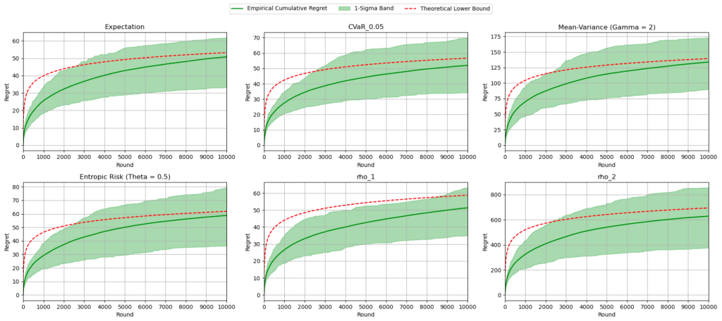
The red curve indicates the theoretical asymptotic lower bound, and each diagram reflects the algorithm running for a fixed $10$ -armed Bernoulli bandit, with different risk functionals, even combinations of them:
- $\rho_1 = 0.5 \cdot \mathrm{CVaR}_{0.05} + 0.5 \cdot \mathrm{ER}_{0.5}$
- $\rho_2(\nu_p) = \rho_{\mathrm{MV}_{2}}(\nu_p) + \exp(2p)$
And for them all, the asymptotic lower bound lies happily in their $1$ -sigma bands. (Yes, each algorithm was averaged across $100$ runs!)

And with that, we are truly done. Happy lunar new year!

—Joel Kindiak, 16 Feb 26, 1131H
February 17, 2026
Real-Life Hypothesis Tests
These problems arise from my actual experience, but numbers have been fudged to protect confidentiality.

Problem 1 (Population Mean). As I taught my classes, I noticed that students are exceedingly taller than I. My height is 160 cm, so I suspect that the average height $\mu$ of students is not 160 cm. By collecting the heights $x$ cm of 30 randomly chosen students, I obtained the following data:

$\Sigma x = 4840,\quad \Sigma x^2 = 781\, 176.$

Test at the 5% significance level to determine whether my suspicion is justified.
(Click for Solution)

Solution. Let $X$ denote the height of a randomly chosen student in cm, and $\mu = \mathbb E[X]$ .

We first set up the null and alternative hypotheses:

$\mathrm H_0 : \mu = 160,\quad \mathrm H_1 : \mu \neq 160.$

Denote the population variance by $\sigma^2$ and $n = 30$ . Assume $\mathrm H_0$ holds, so that $\mu = 60$ . Since $n \geq 30$ , by the central limit theorem,

$\displaystyle \frac{\bar X_n - \mu}{\sigma / \sqrt{n}} \approx Z \sim \mathcal N(0, 1).$

Since $\sigma^2$ is unknown, we need to estimate it using $s^2$ :

$\displaystyle s^2 = \frac 1{30-1} \left( 781\, 176 - \frac{4840^2}{30} \right) \approx 11.1.$

Furthermore, we estimate $\mu$ using $\bar x$ :

$\displaystyle \bar x = \frac{4840}{30} \approx 161.$

Hence, our calculated test statistic $c$ will be

$\displaystyle c := \frac{\bar x - \mu}{s/\sqrt{n}} = \frac{161.33 - 160}{\sqrt{11.126 / 30}} \approx 2.19.$

Since $n \geq 30$ , $t(n-1) \approx \mathcal N(0, 1)$ , so that using either a $z$ – or a $t$ -test would yield similar results. Denote $T \sim t(n-1)$ and the significance level $\alpha = 0.05$ .
- Using a $z$ -table, $p \leq \alpha \iff |z| \geq 1.96$ .
- Using a $t$ -table, $p \leq \alpha \iff |t| \geq 2.05$ .
Whether we let $z = c$ or $t = c$ , it is true that $p \leq \alpha$ . Therefore, there is sufficient evidence to reject $\mathrm H_0$ and conclude that Joel’s suspicion is justified, i.e. the average height of students is larger than $160$ cm.
Problem 2 (Confidence Intervals). Keep the scenario as Problem 1 but denote the true population mean by $\mu_0$ . Use the $t$ -test for simplicity. Determine the interval of values that $\mu_0$ can take such that there is insufficient evidence to reject the null hypothesis at the 5% significance.

(Click for Solution)

Solution. By definition,

$\displaystyle t = \frac{\bar x - \mu_0}{s / \sqrt n} \quad \iff \quad \mu_0 = \bar x - t \cdot \frac{s}{\sqrt n}.$

We do not reject $\mathrm H_0$ if and only if $p > \alpha = 0.05$ . Therefore,

$p > \alpha \quad \iff \quad |t| < 2.05 =: t_{\alpha/2} \quad \iff \quad -t \in (-t_{\alpha/2}, t_{\alpha/2}).$

Therefore,

$\displaystyle \mu_0 = \bar x - t \cdot \frac{s}{\sqrt n} \in \left( \bar x - t_{\alpha/2} \cdot \frac{s}{\sqrt n}, \ \bar x + t_{\alpha/2} \cdot \frac{s}{\sqrt n}\right).$

Remark 1. We call this calculated interval the $(1-\alpha)$ -confidence interval for $\mu_0$ . Denoting a specific sample $K := \{X_1,\dots, X_n\}$ , let $\bar X_K, S_K^2$ denote the corresponding computed unbiased estimators for $\mu, \sigma^2$ respectively. Then the computed corresponding confidence interval $I_K$ will equal

$I_K = \displaystyle \left( \bar X_K - t_{\alpha/2} \cdot \frac{S_K}{\sqrt n}, \bar X_K + t_{\alpha/2} \cdot \frac{S_K}{\sqrt n}\right).$

Hence, different samples would yield different confidence intervals. Since $K$ is random, so is $I_K$ . Furthermore, defining $T := (\bar X_K - \mu_0)/(S_K/\sqrt n) \sim t(n-1)$ , mimicking the computation above yields

$\mathbb P(\mu_0 \in I_K) = \mathbb P(- t_{\alpha/2} < T < t_{\alpha/2}) = 1-\alpha.$

Thus, we have the following interpretation of a $(1-\alpha)$ -confidence interval: the probability that a randomly chosen confidence interval will contain the (deterministic though unknown) population mean is $(1-\alpha)$ .

Problem 3 (Population Proportion). I went to a nearby café, and noticed that there were more women than men in the café. Out of 50 people present, 32 were women.

I suspect that it is true in general that there were more women than men in Starbucks on average. Test at the 5% significance level to determine whether my suspicion is justified.

(Click for Solution)

Solution. Let $\xi$ be a Bernoulli random variable that represents the gender of a person. Here $\xi = 0$ denotes that the person is a man and $\xi = 1$ denotes that the person is a woman. Denote $p := \mathbb E[\xi]$ , which yields the proportion of women in the café.

We first set up the null and alternative hypotheses:

$\mathrm H_0 : p = 0.5,\quad \mathrm H_1 : p > 0.5.$

Assume $\mathrm H_0$ holds, so that $p = 0.5$ . We next estimate $p$ using $\bar \xi_n$ :

$\displaystyle \bar \xi_n = \frac{32}{50} = 0.64.$

Since $n = 50 \geq 30$ and $np(1-p) = 12.5 \geq 10$ , by the central limit theorem,

$\displaystyle \frac{\bar \xi_n - p}{\sqrt{p(1-p)}/\sqrt n} \approx Z \sim \mathcal N(0, 1).$

Hence, our calculated test statistic, the $z$ -value, will be as follows:

$\displaystyle z := \frac{0.64 - 0.5}{ \sqrt{0.5 (1-0.5 )}/\sqrt{50} } \geq 1.97.$

Using a $z$ -table, $p := \mathbb P(Z > z) < 0.05 = \alpha \iff z > 1.645$ , which holds. Therefore, there is sufficient evidence to reject $\mathrm H_0$ and conclude that Joel’s suspicion is justified, i.e. there are more women than men on average.

Problem 4 (Goodness-of-Fit). A total of 750 students took an assessment worth $10$ marks. For each $k = 1, 2, \dots, 10$ , let $f(k)$ denote the number of students who scored $k$ marks out of 10. We have the following data:

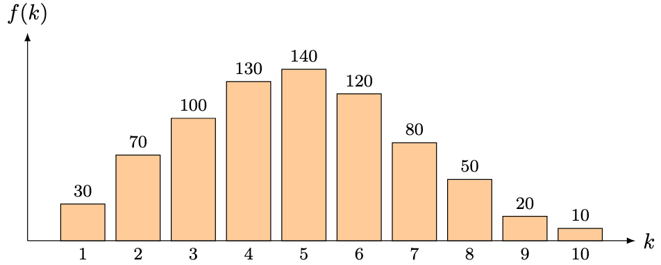
Assuming that scores are continuous, determine at the 5% significance level if the scores can be well-approximated using a normal distribution.

(Click for Solution)

Solution. Let $X$ denote the score of a randomly chosen student with $\mu = \mathbb E[X]$ and $\sigma^2 = \mathrm{Var}(X)$ . We first set up the null and alternative hypotheses:

$\mathrm H_0 : X \sim \mathcal N(\mu, \sigma^2),\quad \mathrm H_1 : X \not \sim \mathcal N(\mu, \sigma^2).$

We first estimate $\mu$ and $\sigma^2$ using $\bar x$ and $s^2$ respectively. Denoting the scores by $x$ , the summary statistics are

$\Sigma x = 3600,\quad \Sigma x^2 = 21\, 600.$

Hence,

$\displaystyle \bar x = \frac{3650}{750} \approx 4.87,\quad s^2 = \frac 1{749} \left(21\, 600 - \frac{3600^2}{750}\right) \approx 4.12.$

Now we assume $\mathrm H_0$ holds, so that $X \sim \mathcal N(4.87, 4.12)$ . Denoting

$p_k := \mathbb P(k - 0.5 < X < k + 0.5),$

we will use the test statistic

$\displaystyle W = \sum_{k=1}^{10} \frac{ (f(k) - 750p_k)^2 }{ 750p_k } \sim \chi^2(9),$

which follows a $\chi^2$ -distribution with $10-1 = 9$ degrees of freedom. For a proof for why this distribution works, refer to this document. Using relevant $z$ -table look-up values (or a spreadsheet application), we obtain the following values for $E_k \equiv 750 p_k$ (rounded to the nearest integer for readability, but whose original value we use in the final computation):

$\begin{aligned} E_1 = 25 \quad E_2 = 55 \quad E_3 &= 96 \quad E_4 = 133 \quad E_5 = 146 \\ E_6 = 125 \quad E_7 = 85 \quad E_8 &= 45 \quad E_9 = 19 \quad E_{10} = 6 \end{aligned}$

Piecing all of the values together,

$\displaystyle w = \sum_{k=1}^{10} \frac{ (f(k) - 750 p_k)^2}{ 750 p_k } \approx 1.97.$

Using a $\chi^2$ -table, $p := \mathbb P(W > w) < 0.05 = \alpha \iff w > 18.3$ , which does not hold. Therefore, there is (woefully) insufficient evidence to reject $\mathrm H_0$ and we cannot conclude that $X$ does not follow a normal distribution.

Problem 5 (Population Variance). Using the data in Problem 4, and assuming that the scores are normally distributed, test at the 5% significance level to determine if the standard deviation of assessment scores is greater than 2.

(Click for Solution)

Solution. We first set up the null and alternative hypotheses:

$\mathrm H_0 : \sigma^2 = 4, \quad \mathrm H_1 : \sigma^2 > 4.$

We use the test statistic $W := (n-1) S^2 / \sigma^2 \sim \chi(n-1)$ :

$\displaystyle w = \frac{ (750 - 1) \cdot 4.12105 }{ 4 } \approx 772.$

Using a spreadsheet application, $\mathbb P(W > w) < 0.05 = \alpha \iff w > 686$ . Therefore, there is sufficient evidence to reject $\mathrm H_0$ and conclude that $\sigma^2 > 4$ , which implies $\sigma > 2$ .

—Joel Kindiak, 4 Dec 25, 1915H
February 13, 2026
The Exponential Family
Recall that if $\lambda > 0$ and $X_n \sim \mathrm{Geom}(\lambda/n)$ , for any $x \geq 0$ ,

$\displaystyle \lim_{n \to \infty} \mathbb P\left( \frac {X_n}n > x \right) = e^{-\lambda x}.$

Definition 1. A continuous random variable is said to follow an exponential distribution with rate parameter $\lambda > 0$ , denoted $X \sim \mathrm{Exp}(\lambda)$ , if

$\mathbb P(X > x) = e^{-\lambda x}.$

Suppose $X \sim \mathrm{Exp}(\lambda)$ .

Problem 1. Prove the following properties:
- $f_X(x) = \lambda e^{-\lambda x} \cdot \mathbb I_{[0,\infty)}(x)$ ,
- $\mathbb E[X] = 1/\lambda$ ,
- $\mathrm{Var}(X) = 1/\lambda^2$ ,
- $X$ satisfies the memoryless property.
(Click for Solution)

Solution. The c.d.f. $F_X$ of $X$ for $x > 0$ is given by

$F_X(x) = \mathbb P(X \leq x) = 1 - \mathbb P(X > x) = 1 - e^{-\lambda x}.$

Hence,

$\displaystyle f_X(x) = \frac{\mathrm d}{\mathrm dx}(F_X(x)) = \frac{\mathrm d}{\mathrm dx} (1- e^{-\lambda x}) = \lambda e^{-\lambda x}.$

For the second result, we use the tail-probability characterisation of the expectation, where the interchange of integrals is valid by Fubini’s theorem:

$\begin{aligned} \mathbb E[X] &= \int_{-\infty}^{\infty} x f_X(x)\, \mathrm dx \\ &= \int_{0}^{\infty} \int_0^x f_X(x)\, \mathrm dy\, \mathrm dx \\ &= \int_{0}^{\infty} \int_{y}^\infty f_X(x) \, \mathrm dx \, \mathrm dy \\ &= \int_{0}^{\infty} \mathbb P(X > y) \, \mathrm dy. \end{aligned}$

Hence, for $X \sim \mathrm{Exp}(\lambda)$ ,

$\begin{aligned} \mathbb E[X] &= \int_{0}^{\infty} e^{-\lambda y}\, \mathrm dy = \frac 1{\lambda} \cdot [-e^{-\lambda y}]_0^\infty = \frac 1{\lambda} \cdot (0 - (-1)) = \frac 1{\lambda}. \end{aligned}$

For the variance, we adopt a similar approach:

$\begin{aligned} \mathbb E[X^2] &= \int_{-\infty}^{\infty} 2y \cdot \mathbb P(X > y) \, \mathrm dy \\ &= \int_{0}^{\infty} 2y \cdot e^{-\lambda y} \, \mathrm dy \\ &= \frac 2{\lambda} \int_0^\infty y e^{-\lambda y}\, \mathrm dy \\ &= \frac 2{\lambda} \cdot \mathbb E[X] = \frac 2{\lambda^2}. \end{aligned}$

Therefore,

$\displaystyle \mathrm{Var}(X) = \mathbb E[X^2] - \mathbb E[X]^2 = \frac{2}{\lambda^2} - \frac 1{\lambda^2} = \frac{1}{\lambda^2}.$

For the memoryless property,

$\begin{aligned} \mathbb P(X > s + t \mid X > t) &= \frac{\mathbb P(X > s + t, X > t)}{\mathbb P(X > t)} \\ &= \frac{\mathbb P(X > s+t)}{\mathbb P(X > t)} = \frac{e^{-\lambda(s+t)}}{e^{-\lambda t}} \\ &= e^{-\lambda s} = \mathbb P(X > s).\end{aligned}$

Problem 2. Suppose $Y \sim \mathrm{Exp}(\mu)$ is independent to $X$ .
- Calculate the distribution of $\min\{X, Y\}$ .
- If $\lambda = \mu$ , evaluate the p.d.f. of $X + Y$ .
(Click for Solution)

Solution. Denoting $W := \min\{X, Y\}$ ,

$\begin{aligned} \mathbb P(W > w) &= \mathbb P(X > w, Y > w) \\ &= \mathbb P(X > w) \cdot \mathbb P(Y > w)\\&= e^{-\lambda w} \cdot e^{-\mu w} \\ &= e^{-(\lambda + \mu) w}. \end{aligned}$

Hence, $\min\{X, Y\} = W \sim \mathrm{Exp}(\lambda + \mu)$ . To evaluate the p.d.f. of $U:= X+ Y$ , we compute the convolution of their individual p.d.f.s:

$\begin{aligned} f_U(u) &= (f_X * f_Y)(u) \\ &= \int_0^u f_X(x) \cdot f_Y(u-x)\, \mathrm dx \\ &= \int_0^u \lambda e^{-\lambda x} \cdot \mu e^{-\mu(u - x)}\, \mathrm dx \\ &= \lambda \cdot \mu \cdot e^{-\mu u} \cdot \int_0^u e^{-(\lambda - \mu) x} \, \mathrm dx \\ &= \lambda^2 \cdot e^{-\lambda u} \cdot \int_0^u 1 \, \mathrm dx \\ &= \lambda^2 \cdot u \cdot e^{-u}. \end{aligned}$

Definition 2. A continuous random variable $X$ is said to follow a gamma distribution with shape parameter $\alpha > 0$ and rate parameter $\lambda > 0$ , denoted $X \sim \Gamma( \alpha, \lambda)$ if it has a p.d.f. given by

$\displaystyle f_X(x) = \frac{\lambda^\alpha}{\Gamma(\alpha)} \cdot x^{\alpha - 1} \cdot e^{-\lambda x}.$

Problem 3. Prove the following properties:
- if $X \sim \Gamma(\alpha, \lambda)$ , then $\mathbb E[X] = \alpha/\lambda$ , $\mathrm{Var}(X) = \alpha/\lambda^2$ ,
- if $X_i \sim \Gamma(\alpha_i, \lambda)$ are i.i.d., then $\sum_{i=1}^n X_i \sim \Gamma(\sum_{i=1}^n \alpha_i, \lambda)$ ,
- if $X \sim \Gamma(\alpha, \lambda)$ and $c > 0$ , then $cX \sim \Gamma(\alpha, \lambda/c)$ .
(Click for Solution)

Solution. Suppose $Y \sim \Gamma(\alpha + 1,\lambda)$ . By definition of the expectation,

$\begin{aligned} \mathbb E[X^n] &= \int_0^\infty x^n \cdot \frac{\lambda^\alpha}{\Gamma(\alpha)} \cdot x^{\alpha - 1} \cdot e^{-\lambda x}\, \mathrm dx \\ &= \frac {\alpha \cdot (\alpha+1) \cdot \cdots \cdot (\alpha +n-1)}{\lambda^n} \cdot \int_0^\infty \frac{\lambda^{\alpha+n}}{\Gamma(\alpha+1)} \cdot x^{(\alpha + n) - 1} \cdot e^{-\lambda x}\, \mathrm dx \\ &= \frac{\alpha \cdot (\alpha+1) \cdot \cdots \cdot (\alpha +n-1)}{\lambda^n} \cdot \int_0^\infty f_Y(x)\, \mathrm dx \\ &= \frac{\alpha \cdot (\alpha+1) \cdot \cdots \cdot (\alpha +n-1)}{\lambda^n} . \end{aligned}$

Hence, $\mathbb E[X] = \alpha/\lambda$ , and

$\begin{aligned} \mathrm{Var}(X) &= \mathbb E[X^2] - \mathbb E[X]^2 = \frac{\alpha \cdot (\alpha+1)}{\lambda^2} - \frac{\alpha^2}{\lambda^2} = \frac{\alpha}{\lambda^2}. \end{aligned}$

We prove the second result by induction. Suppose $X \sim \Gamma(\alpha, \lambda)$ and $Y \sim \Gamma (\beta, \lambda)$ are independent. To evaluate the p.d.f. of $U:= X+ Y$ , we compute the convolution of their individual p.d.f.s:

$\begin{aligned} f_U(u) &= (f_X * f_Y)(u) \\ &= \int_0^u f_X(x) \cdot f_Y(u-x)\, \mathrm dx \\ &= \int_0^u \frac{\lambda^\alpha}{\Gamma(\alpha)} \cdot x^{\alpha - 1} \cdot e^{-\lambda x} \cdot \frac{\lambda^\beta}{\Gamma(\beta)} \cdot (u-x)^{\beta - 1} \cdot e^{-\lambda (u-x)}\, \mathrm dx \\ &= \frac{\lambda^{\alpha + \beta}}{\Gamma(\alpha) \cdot \Gamma(\beta)} \cdot \int_0^u x^{\alpha - 1} \cdot (u-x)^{\beta - 1} \cdot e^{-\lambda u}\, \mathrm dx \\ &= \frac{\lambda^{\alpha + \beta}}{\Gamma(\alpha) \cdot \Gamma(\beta)} \cdot \int_0^1 (ut)^{\alpha - 1} \cdot (u-ut)^{\beta - 1} \cdot e^{-\lambda u}\cdot u\, \mathrm dt \\ &= \frac{\lambda^{\alpha + \beta}}{\Gamma(\alpha + \beta)} \cdot u^{(\alpha+\beta) -1}\cdot e^{-\lambda u} \cdot \frac{\Gamma(\alpha + \beta)}{\Gamma(\alpha) \cdot \Gamma(\beta)} \cdot \int_0^1 t^{\alpha - 1} \cdot (1-t)^{\beta - 1} \, \mathrm dt \\ &= \frac{\lambda^{\alpha + \beta}}{\Gamma(\alpha + \beta)} \cdot u^{(\alpha+\beta) -1}\cdot e^{-\lambda u}. \end{aligned}$

Therefore, $W \sim \Gamma(\alpha +\beta, \lambda)$ . Inductively, if $X_i \sim \Gamma(\alpha_i, \lambda)$ are i.i.d.,

$\displaystyle \sum_{i=1}^{k+1} X_i = \sum_{i=1}^{k} X_i + X_{k+1} \sim \Gamma \left( \sum_{i=1}^{k} \alpha_i + \alpha_{k+1}, \lambda \right) = \Gamma \left( \sum_{i=1}^{k+1} \alpha_i, \lambda \right).$

For the final property, denoting $V := cX$ ,

$\begin{aligned} f_{V}(v) = f_{cX}(v) &= \frac 1c \cdot f_X\left( \frac vc \right) \\ &= \frac 1c \cdot \frac{\lambda^\alpha}{\Gamma(\alpha)} \cdot \left( \frac vc \right)^{\alpha - 1} \cdot e^{-\lambda v/c} \\ &= \frac{(\lambda /c)^\alpha}{\Gamma(\alpha)} \cdot v^{\alpha - 1} \cdot e^{-(\lambda /c) v}. \end{aligned}$

Hence, $cX = V \sim \Gamma(\alpha, \lambda / c)$ .

Given probability distributions $\mathbb Q_1, \mathbb Q_2$ , write $\mathbb Q_1 =\mathbb Q_2$ if there exists a random variable $X$ such that $X \sim \mathbb Q_1$ and $X \sim \mathbb Q_2$ .

Problem 4. Prove the following properties:
- $\mathrm{Exp}(\lambda) = \Gamma(1, \lambda)$ ,
- $\Gamma(\nu/2, 1/2) = \chi^2(\nu)$ ,
- for i.i.d. $X_1,\dots, X_n \sim \mathrm{Exp}(\lambda)$ , $\sum_{i=1}^n X_i \sim \Gamma(n, \lambda),\bar X \sim \Gamma(n, \lambda/n)$ ,
- for any fixed $c > 0$ , if $W \sim \chi^2(\nu)$ , then $cW \sim \Gamma(\nu/2, 1/(2c))$ .
(Click for Solution)

Solution. We note that if $X \sim \Gamma( 1,\lambda)$ , since $\Gamma(1) = 0! = 1$ ,

$\displaystyle f_X(x) = \frac{\lambda}{\Gamma(1)} \cdot x^{1 - 1} \cdot e^{-\lambda x} = \lambda e^{-\lambda x},$

so that $X \sim \mathrm{Exp}(1, \lambda)$ . If $X \sim \Gamma( \nu/2, 1/2)$ , then

$\displaystyle f_X(x) = \frac{(1/2)^{\nu/2}}{\Gamma(\nu/2)} \cdot x^{\nu/2 - 1} \cdot e^{-x/2} = \frac{1}{2^{\nu/2} \cdot \Gamma(\nu/2)} \cdot x^{\nu/2 - 1} \cdot e^{-x/2}.$

The last two results are immediate corollaries of Problem 3.

These probability distributions are examples of the exponential family of probability distributions.

—Joel Kindiak, 4 Aug 25, 1356H
January 9, 2026
The Geometric Distribution

Definition 1. For $K \subseteq \mathbb R$ , a random variable $X : \Omega \to K$ satisfies the memoryless property if the following holds: for any $s, t \in K$ ,

$\displaystyle \mathbb P(X > s + t \mid X > t) = \mathbb P(X > s).$

Problem 1. If $K = \mathbb N^+$ and $X$ satisfies the memoryless property, compute an expression for $\mathbb P(X = x)$ in terms of $p := \mathbb P(X = 1)$ .

(Click for Solution)

Solution. Define the function $G$ by $G(x):= \mathbb P(X > x)$ . By the definition of conditional probability,

$\begin{aligned} G(s+t) = \mathbb P(X > s+t) &= \mathbb P(X > s +t, X>t) \\ &= \mathbb P(X > s +t \mid X>t) \cdot \mathbb P(X > t) \\ &= \mathbb P(X > s) \cdot \mathbb P(X > t) \\ &= G(s) \cdot G(t). \end{aligned}$

Therefore, $G(x) = a^x$ for some $a > 0$ . In particular,

$a = G(1) = \mathbb P(X > 1) = 1 - \mathbb P(X=1) = 1-p.$

Therefore, $G(x) = (1-p)^x$ , so that

$\begin{aligned} \mathbb P(X=x) &= \mathbb P(X > x-1) - \mathbb P(X > x) \\ &= (1-p)^{x-1} - (1-p)^x \\ &= (1-p)^{x-1} \cdot (1 - (1-p)) \\ &= (1-p)^{x-1} \cdot p. \end{aligned}$

Definition 2. A discrete random variable $X : \Omega \to \mathbb N^+$ is said to follow a geometric distribution with success probability $p$ , denoted $X \sim \mathrm{Geom}(p)$ , if

$\displaystyle \mathbb P(X = x) = (1-p)^{x-1} \cdot p,\quad x \in \mathbb N^+.$

Suppose $X \sim \mathrm{Geom}(p)$ .

Problem 2. Prove that $X$ satisfies the memoryless property.

(Click for Solution)

Solution. Using a geometric series,

$\begin{aligned} \mathbb P(X > x) &= \sum_{k=x+1}^\infty \mathbb P(X = k) \\ &= \sum_{k=x+1}^\infty (1-p)^{k-1} \cdot p \\ &= \frac{p\cdot (1-p)^x}{1 - (1-p)} = (1-p)^x. \end{aligned}$

By the definition of conditional probability,

$\begin{aligned} \mathbb P(X > s +t \mid X>t) &= \frac{\mathbb P(X > s +t, X>t)}{\mathbb P(X > t)} \\ &= \frac{\mathbb P(X > s +t)}{\mathbb P(X > t)} \\ &= \frac{(1-p)^{s+t}}{(1-p)^t} \\ &= (1-p)^s = \mathbb P(X > s). \end{aligned}$

Problem 3. Prove that $\displaystyle \mathbb E[X] = \sum_{x = 0}^\infty \mathbb P(X > x)$ . Hence, evaluate $\mathbb E[X]$ and $\mathrm{Var}(X)$ .

(Click for Solution)

Solution. By interchanging sums,

$\begin{aligned} \mathbb E[X] &= \sum_{x = 0}^\infty x \cdot \mathbb P(X = x) = \sum_{x=0}^\infty \sum_{y=0}^{x-1} \mathbb P(X = x) \\ &= \sum_{y=0}^\infty \sum_{x=y+1}^\infty \mathbb P(X = x) = \sum_{y=0}^\infty \mathbb P(X > y) = \sum_{x = 0}^\infty \mathbb P(X > x). \end{aligned}$

Hence, using the calculations in Problem 2,

$\displaystyle \mathbb E[X] = \sum_{x=0}^\infty (1-p)^x = \frac{1}{1-(1-p)} = \frac 1p.$

For the variance, we first compute $\mathbb E[X^2]$ . Observe that

$\displaystyle \sum_{y=0}^{x-1} (2y + 1) = x^2.$

Therefore, by interchanging sums,

$\begin{aligned} \mathbb E[X^2] &= \sum_{x = 0}^\infty x^2 \cdot \mathbb P(X = x) \\ &= \sum_{x=0}^\infty \sum_{y=0}^{x-1} (2y + 1) \cdot \mathbb P(X = x) \\ &= \sum_{y=0}^\infty \sum_{x=y+1}^\infty (2y + 1) \cdot \mathbb P(X = x) \\ &= \sum_{y=0}^\infty \left( (2y + 1) \cdot \sum_{x=y+1}^\infty (1-p)^{x-1} \cdot p \right) \\ &= \sum_{y=0}^\infty \left( (2y + 1) \cdot \frac{(1-p)^y}{1 - (1-p)} \cdot p \right) \\ &= \frac 1p \cdot \sum_{y=0}^\infty \left( (2y + 1) \cdot (1-p)^y \cdot p \right) \\ &= \frac 1p \cdot \left( p + (1-p) \cdot \left( 2 \cdot \sum_{y=1}^\infty y\cdot \mathbb P(X = y ) + \sum_{y=1}^\infty \mathbb P(X = y ) \right) \right) \\ &= \frac 1p \cdot \left( p + (1-p) \cdot \left( \frac 2p + 1 \right) \right) \\ &= 1 + \left( \frac 1p - 1 \right) \cdot \left( \frac 2p + 1 \right) \\ &= 1 + \frac 2{p^2} + \frac 1p - \frac 2p - 1 = \frac {2-p}{p^2}. \end{aligned}$

Therefore,

$\begin{aligned} \mathrm{Var}(X) &= \mathbb E[X^2] -\mathbb E[X]^2 = \frac {2-p}{p^2} - \frac 1{p^2} = \frac{1-p}{p^2}. \end{aligned}$

Problem 4. If $Y \sim \mathrm{Geom}(q)$ is independent of $X$ , compute the distribution of $\min\{X, Y\}$ .

(Click for Solution)

Solution. Denote $W := \min \{X, Y\}$ . Then

$\begin{aligned} \mathbb P(W > w) &= \mathbb P(\min\{X,Y\} > w) \\ &= \mathbb P(X > w, Y > w) \\ &= \mathbb P(X > w) \cdot \mathbb P(Y > w) \\ &= (1-p)^w \cdot (1-q)^w = ((1-p)(1-q))^w. \end{aligned}$

Therefore, $\min\{X, Y\} \sim \mathrm{Geom}(1-(1-p)(1-q))$ .

Problem 5. Fix $\lambda > 0$ . Suppose $X_n \sim \mathrm{Geom}(\lambda /n)$ . For any $x > 0$ , evaluate

$\displaystyle \lim_{n \to \infty} \mathbb P \left( \frac {X_n}n > x \right) .$

(Click for Solution)

Solution. Using the tail-probability,

$\begin{aligned} \lim_{n \to \infty} \mathbb P \left( \frac {X_n}n > x \right) &= \lim_{n \to \infty} \mathbb P(X_n > nx) \\ &= \lim_{n \to \infty} \left( 1 - \frac{\lambda}n \right)^{nx} \\ &= \left( \lim_{n \to \infty} \left( 1 - \frac{\lambda}n \right)^{n} \right)^x \\ &= (e^{-\lambda})^x = e^{-\lambda x}. \end{aligned}$

—Joel Kindiak, 3 Aug 25, 0004H

January 6, 2026
The Gaussian Integral

Problem 1. Evaluate the Gaussian integral $\displaystyle \int_{-\infty}^{\infty} e^{-x^2}\, \mathrm dx$ .

(Click for Solution)

Solution. Since $e^{-x^2}$ is even in $x$ ,

$\displaystyle \int_{-\infty}^{\infty} e^{-x^2}\, \mathrm dx = 2 \cdot \int_{0}^{\infty} e^{-x^2}\, \mathrm dx.$

For the right-hand side,

$\begin{aligned}\left( \int_{0}^{\infty} e^{-x^2}\, \mathrm dx \right)^2 &= \left( \int_{0}^{\infty} e^{-x^2}\, \mathrm dx \right) \cdot \left( \int_{0}^{\infty} e^{-y^2}\, \mathrm dy \right) \\ &= \int_0^\infty e^{-x^2} \cdot \left( \int_0^\infty e^{-y^2}\, \mathrm dy \right)\, \mathrm dx \\ &= \int_0^\infty e^{-x^2} \cdot \left( \int_0^\infty e^{-u^2x^2} \cdot x\, \mathrm du \right)\, \mathrm dx \\ &= \int_0^\infty \int_0^\infty xe^{-x^2(u^2+1)} \, \mathrm du\, \mathrm dx. \end{aligned}$

By Fubini’s theorem,

$\begin{aligned}\left( \int_{0}^{\infty} e^{-x^2}\, \mathrm dx \right)^2 &= \int_0^\infty \int_0^\infty xe^{-x^2(u^2+1)} \, \mathrm du\, \mathrm dx\\ &= \int_0^\infty \int_0^\infty xe^{-x^2(u^2+1)} \, \mathrm dx\, \mathrm du \\ &= \int_0^\infty \left[ -\frac 1{2(u^2+1)} \cdot e^{-x^2(u^2+1)} \right]_0^\infty\, \mathrm du \\ &= \int_0^\infty \frac 1{2(u^2+1)}\, \mathrm du \\ &= \frac 12 \cdot [\tan^{-1}(u)]_0^{\infty} \\ &= \frac 12 \cdot \frac{\pi}2 = \frac{\pi}{4}. \end{aligned}$

Taking square roots,

$\displaystyle \int_{0}^{\infty} e^{-x^2}\, \mathrm dx = \frac{\sqrt{\pi}}{2} \quad \Rightarrow \quad \int_{-\infty}^{\infty} e^{-x^2}\, \mathrm dx = \sqrt{\pi}.$

This calculation was authored by Hirokazu Iwasawa.

—Joel Kindiak, 26 Jul 25, 2156H

January 2, 2026
The Poisson Distribution

Definition 1. The random variable $X : \Omega \to \mathbb N_0$ follows a Poisson distribution with rate parameter $\lambda > 0$ , denoted $X \sim \mathrm{Pois}(\lambda)$ , if

$\displaystyle \mathbb P(X=x) = c_\lambda \cdot \frac{\lambda^x}{x!}$

for some $c_\lambda > 0$ .

Problem 1. Evaluate $c_\lambda$ .

(Click for Solution)

Solution. We require $\sum_{x = 0}^\infty \mathbb P(X=x) = 1$ :

$\begin{aligned}1 = \sum_{x = 0}^\infty \mathbb P(X=x) &= \sum_{x =0}^\infty c_\lambda \cdot \frac{\lambda^x}{x!} = c_\lambda \cdot \sum_{x = 0}^\infty \frac{\lambda^x}{x!} = c_\lambda \cdot e^{\lambda}. \end{aligned}$

Therefore, $c_\lambda = e^{-\lambda}$ .

Problem 2. Evaluate $\mathbb E[X]$ and $\mathrm{Var}(X)$ .

(Click for Solution)

Solution. By definition of the expectation,

$\begin{aligned} \mathbb E[X] &= \sum_{x = 0}^\infty x \cdot \mathbb P(X=x) \\ &= \sum_{x = 1}^\infty x \cdot c_\lambda \cdot \frac{\lambda^x}{x!} \\ &= \lambda \cdot \sum_{x = 1}^\infty c_\lambda \cdot \frac{\lambda^{x-1}}{(x-1)!} \\ &= \lambda \cdot \sum_{x = 0}^\infty c_\lambda \cdot \frac{\lambda^{x}}{x!} = \lambda \cdot 1 = \lambda. \end{aligned}$

For the variance, we compute the term

$\begin{aligned}\mathbb E[X(X-1)] &= \sum_{x = 0}^\infty x(x-1) \cdot \mathbb P(X=x) \\ &= \sum_{x = 2}^\infty x(x-1) \cdot c_\lambda \cdot \frac{\lambda^x}{x!} \\ &= \lambda^2 \cdot \sum_{x = 2}^\infty c_\lambda \cdot \frac{\lambda^{x-2}}{(x-2)!} \\ &= \lambda^2 \cdot 1 = \lambda^2. \end{aligned}$

Therefore,

$\begin{aligned} \mathrm{Var}(X) &= \mathbb E[X^2] - \mathbb E[X]^2 \\ &= \mathbb E[X(X-1)] + \mathbb E[X] - \mathbb E[X]^2 \\ &= \lambda^2 + \lambda - \lambda^2 = \lambda.\end{aligned}$

Problem 3. Given that $X \sim \mathrm{Pois}(\lambda)$ and $Y \sim \mathrm{Pois}(\mu)$ are independent, determine the distribution of $X + Y$ .

(Click for Solution)

Solution. Denoting $W := X+Y$ , we take the discrete convolution of the p.d.f.s of $X,Y$ to obtain

$\begin{aligned}f_W (w) &= \sum_{x = 0}^w f_X(x) \cdot f_Y(w-x) \\ &= \sum_{x=0}^w c_\lambda \cdot \frac{\lambda^x}{x!} \cdot c_\mu \cdot \frac{\lambda^{w-x}}{(w-x)!} \\ &= \sum_{x=0}^w c_\lambda \cdot \frac{\lambda^x}{x!} \cdot c_\mu \cdot \frac{\mu^{w-x}}{(w-x)!} \\ &= c_\lambda \cdot c_\mu \cdot \sum_{x=0}^w \frac{\lambda^x}{x!} \cdot \frac{\mu^{w-x}}{(w-x)!} \\ &= c_\lambda \cdot c_\mu \cdot \frac 1{w!} \cdot \sum_{x=0}^w \frac{w!}{x! \cdot (w-x)!} \cdot \lambda^x \cdot \mu^{w-x} \\ &= c_\lambda \cdot c_\mu \cdot \frac 1{w!} \cdot \sum_{x=0}^w {w \choose x} \cdot \lambda^x \cdot \mu^{w-x} \\ &= c_\lambda \cdot c_\mu \cdot \frac {(\lambda + \mu)^w}{w!}.\end{aligned}$

Furthermore, $c_\lambda \cdot c_\mu = e^{-\lambda} \cdot e^{\mu} = e^{-(\lambda + \mu)} = c_{\lambda + \mu}$ . Hence,

$\displaystyle \mathbb P(X+Y = w) = c_{\lambda + \mu} \cdot \frac{(\lambda + \mu)^w}{w!},$

so that $X +Y \sim \mathrm{Pois}(\lambda + \mu)$ .

Problem 4. Fix $\lambda > 0$ . Suppose $X_n \sim \mathrm{Bin}(n, \lambda/n)$ and $Y \sim \mathrm{Pois}(\lambda)$ . Prove that $f_{X_n} \to f_Y$ .

(Click for Solution)

Solution. Fix $y \in \mathbb N_0$ . For each $n$ ,

$\begin{aligned} f_{X_n}(y) &= {n \choose y} \left(1 - \frac{\lambda}{n}\right)^{n-y} \left( \frac{\lambda}n \right)^y \\ &= \frac{n(n-1) \cdot \dots \cdot (n-y+1)}{y!} \cdot \frac{\lambda^y }{n^y } \cdot \left(1 - \frac{\lambda}{n}\right)^{n-y} \\ &= \frac{n}{n} \cdot \frac{n-1}{n} \cdot \cdots \cdot \frac{n-y+1}n \cdot \left(1 - \frac{\lambda}{n}\right)^{-y} \cdot \left(1 - \frac{\lambda}{n}\right)^{n} \cdot \frac{\lambda^y }{y! } \end{aligned}$

Taking $n \to \infty$ ,

$\displaystyle \lim_{n \to \infty} f_{X_n}(y) = 1 \cdot 1 \cdot e^{-\lambda} \cdot \frac{\lambda^y}{y!} = e^{-\lambda} \cdot \frac{\lambda^y}{y!} = f_Y(y).$

—Joel Kindiak, 1 Aug 25, 1751H

December 30, 2025
Proving Feynman’s Trick
Feynman’s trick in differentiating under the integral sign has been creatively wielded to evaluate otherwise intractable integrals. In this exercise, we prove Feynman’s trick and use it to evaluate the seemingly intractable Dirichlet integral

$\displaystyle \int_{-\infty}^{\infty} \frac{\sin x}{x}\, \mathrm dx.$

Let $(\Omega, \mathcal F, \mathbb R)$ be a measure space and $f : \Omega \times [a, b] \to \mathbb R$ be a function such that for each $t \in [a, b]$ , $f( \cdot, t)$ is measurable.

Problem 1. Suppose the following conditions:
- For any $\omega \in \Omega$ , $f(\omega, \cdot)$ is continuous.
- There exists some non-negative integrable $g : \Omega \to \mathbb R$ such that for any $(\omega, t) \in \Omega \times [a, b]$ , $|f( \omega ,t)| \leq g(\omega)$ .
Prove that the map $F : [a, b] \to \mathbb R$ defined by $\displaystyle F(t) : = \int_{\Omega} f(\cdot , t)\, \mathrm d\mu$ is continuous.

(Click for Solution)

Solution. Fix $t_n \to t$ . For any $\omega \in \Omega$ , since $f(\omega, \cdot)$ is continuous,

$f(\omega, t_n) \to f(\omega, t),$

so that $f(\cdot, t_n) \to f(\cdot, t)$ pointwise. Furthermore,

$\displaystyle \int_{\Omega} |f(\cdot, t)|\, \mathrm d\mu \leq \int_{\Omega} g\, \mathrm d\mu < \infty,$

so that $f(\cdot, t_n)$ and $f(\cdot, t)$ are all integrable.

Since $g$ is integrable, by Lebesgue’s dominated convergence theorem,

$\displaystyle F(t_n) = \lim_{n \to \infty} \int_{\Omega} f(\cdot , t_n)\, \mathrm d\mu= \int_{\Omega} f(\cdot , t)\, \mathrm d\mu = F(t),$

so that $F$ is continuous, as required.

Problem 2. Suppose the following conditions:
- There exists some $t_0 \in [a, b]$ such that $f(\cdot, t_0)$ is integrable.
- For each $\omega \in \Omega$ , $f(\omega, \cdot)$ is differentiable with derivative at $t_0$ denoted by $\frac{\partial f}{\partial t}(\omega,t_0)$ .
- There exists some non-negative integrable $g : \Omega \to \mathbb R$ such that for any $(\omega, t) \in \Omega \times [a, b]$ , $\left|\frac{\partial f}{\partial t} (\omega,t) \right| \leq g( \omega )$ .
Prove that the map $F : [a, b] \to \mathbb R$ defined by $\displaystyle F(t) : = \int_{\Omega} f(\cdot, t)\, \mathrm d\mu$ is differentiable on $[a, b]$ and

$\displaystyle F'(t) = \frac{\mathrm d}{\mathrm dt} \int_{\Omega} f(\omega, t)\, \mathrm d\mu(\omega) = \int_{\Omega} \frac{\partial f}{\partial t}(\omega, t)\, \mathrm d\mu(\omega).$

(Click for Solution)

Solution. We first check that $F$ is well-defined. By hypothesis, $F(t_0)$ is well-defined. Fix $t \in [a, b]$ . By the mean value theorem, there exists $c$ between $t_0$ and latex t$ such that

$\displaystyle \frac{ |f(\omega, t) - f(\omega, t_0)| }{ |t - t_0| } = \left| \frac{ \partial f }{ \partial t} (\omega, c) \right| \leq g(\omega).$

By performing more analysis, $f(\cdot, t)$ is integrable, so that $F(t)$ is well-defined.

Now fix $\omega \in \Omega$ . For any $t_n \to t$ , since each $f(\cdot, t_n) - f(\cdot, t)$ is measurable,

$\displaystyle \frac{\partial f}{\partial t}(\omega, t) := \lim_{n \to \infty} \underbrace{ \frac{f(\omega, t_n) - f(\omega, t)}{ t_n - t} }_{\varphi_n(\omega)}$

is measurable. Furthermore, $\varphi_n \to \frac{\partial f}{\partial t} (\cdot, t)$ pointwise. We claim that $|\varphi_n| \leq g$ , since the mean value theorem gives $c$ between $t_n$ and $t$ such that

$\displaystyle \frac{ | f(\omega, t_n) - f(\omega, t) |}{ | t_n - t | } = \left| \frac{\partial f}{\partial t}(\omega, c) \right| \leq g(\omega).$

By algebruh and the triangle inequality, each $\varphi_n$ is integrable. Hence, by Lebesgue’s dominated convergence theorem,

$\begin{aligned} \lim_{t_n \to t} \int_{\Omega} \frac{f(\omega, t_n) - f(\omega, t)}{t_n - t}\, \mathrm d\mu(\omega) &= \lim_{n \to \infty} \int_{\Omega} \varphi_n\, \mathrm d\mu \\ &= \int_{\Omega} \lim_{n \to \infty} \varphi_n\, \mathrm d\mu = \int_{\Omega} \frac{\partial f}{\partial t} (\cdot, t)\, \mathrm d\mu. \end{aligned}$

On the other hand, by bookkeeping

$\begin{aligned} \frac{ \mathrm d }{ \mathrm dt } F(t) &= \lim_{ t_n \to t } \frac{ F(t_n) - F(t) }{ t_n - t } \\ &= \lim_{t_n \to t} \int_{\Omega} \frac{f(\omega, t_n) - f(\omega, t)}{t_n - t}\, \mathrm d\mu(\omega) \\ &= \int_{\Omega} \frac{\partial f}{\partial t} (\omega, t)\, \mathrm d\mu(\omega). \end{aligned}$

Therefore,

$\displaystyle F'(t) = \frac{\mathrm d}{\mathrm dt} \int f(\omega, t)\, \mathrm d\mu(\omega) = \int \frac{\partial f}{\partial t}(\omega, t)\, \mathrm d\mu(\omega).$

Remark 1. Thanks to Problem 2, our proof that $\mathcal L\{tf'(t)\} = -\mathcal L\{f\}'(s)$ in the study of differential equations becomes a logically correct one.

Problem 3. Use Problem 2 to evaluate $\displaystyle \int_{-\infty}^{\infty} \frac{\sin x}{x}\, \mathrm dx$ .

(Click for Solution)

Solution. Define the function $I$ by

$\displaystyle I(y) := \int_{0}^{\infty} \frac{\sin x}{x} \cdot e^{-xy}\, \mathrm dy$

that satisfies the hypotheses of Problem 2, and our goal is to evaluate $2 \cdot I(0)$ . Applying Problem 2 and integrating by parts,

$\begin{aligned} I'(y) &= \int_{0}^{\infty} \frac{\partial}{\partial y} \left( \frac{\sin x}{x} \cdot e^{-xy} \right) \, \mathrm dx \\ &= \int_{0}^{\infty} \frac{\sin x}{x} \cdot -xe^{-xy} \, \mathrm dx \\ &= -\int_{0}^{\infty} e^{-xy} \cdot \sin x \, \mathrm dx \\ &= -\left[ \frac{e^{-xy}}{(-y)^2 + 1^2} \cdot ((-y) \sin(x) - \cos(x)) \right]_{0}^{\infty} \\ &= -\frac{1}{1+y^2}. \end{aligned}$

Integrating and applying the first fundamental theorem of calculus,

$\displaystyle I(y) = I(0) - \int_0^y \frac{1}{1+y^2}\, \mathrm dy = I(0) - \tan^{-1}(y).$

Since $I$ is continuous,

$\displaystyle \lim_{y \to \infty} I(y) = \int_0^\infty \lim_{y \to \infty} \frac{\sin x}{x} \cdot e^{-xy}\, \mathrm dx = \int_0^\infty 0\, \mathrm dx = 0.$

Taking $y \to \infty$ on all sides, therefore,

$\displaystyle 0 = I(0) - \frac{\pi}{2} \quad \Rightarrow \quad I(0) = \frac{\pi}{2}.$

Therefore, the Dirichlet integral evaluates to

$\displaystyle \int_{-\infty}^{\infty} \frac{\sin x}{x}\, \mathrm dx = 2 \cdot I(0) = \pi.$

—Joel Kindiak, 29 Jul 25, 1319H
December 26, 2025
Binomial Theorem Corollaries

Recall the binomial theorem, which states that for any $n \in \mathbb N$ and $x \in \mathbb R$ ,

$\displaystyle (1 + x)^n = \sum_{k=0}^n {n \choose k} x^k,$

where we define $0^0 := 1$ by convention.

Problem 1. Prove that for any $a, b \in \mathbb R$ ,

$\displaystyle (a + b)^n = \sum_{k=0}^n {n \choose k} a^{n-k} b^k.$

(Click for Solution)

Solution. If $a = 0$ then the result is trivial. If $a > 0$ , then

$\begin{aligned} (a+b)^n &= a^n \cdot \left(1 + \frac ba\right)^n = a^n \cdot \sum_{k=0}^n \left( \frac ba \right)^k \\ &= a^n \cdot \sum_{k=0}^n a^{-k} \cdot b^k = \sum_{k=0}^n a^{n-k} \cdot b^k. \end{aligned}$

Problem 2. Evaluate the sums $\displaystyle \sum_{k=0}^n {n \choose k}$ and $\displaystyle \sum_{k=0}^n (-1)^k {n \choose k}$ .

(Click for Solution)

Solution. By Problem 1,

$\displaystyle (1 + (\pm 1))^n = \sum_{k=0}^n (\pm 1)^k {n \choose k}.$

Therefore, $\displaystyle \sum_{k=0}^n {n \choose k} = (1+1)^n = 2^n$ and $\displaystyle \sum_{k=0}^n (-1)^k {n \choose k} = (1-1)^n = 0$ .

Problem 3. Prove that $\displaystyle \sum_{k \in \mathbb N_0 :\, 2k \leq n} {n \choose 2k} = \sum_{k \in \mathbb N_0 :\, 2k+1 \leq n} {n \choose 2k+1}$ .

(Click for Solution)

Solution. By Problem 2,

$\begin{aligned} 0=\sum_{k=0}^n (-1)^k {n \choose k} &= \sum_{k \in \mathbb N_0 :\, 2k \leq n} (-1)^{2k} {n \choose 2k} + \sum_{k \in \mathbb N_0 :\, 2k+1 \leq n} (-1)^{2k+1} {n \choose 2k+1} \\ &= \sum_{k \in \mathbb N_0 :\, 2k \leq n} {n \choose 2k} - \sum_{k \in \mathbb N_0 :\, 2k+1 \leq n} {n \choose 2k+1}. \end{aligned}$

Therefore,

$\displaystyle \sum_{k \in \mathbb N_0 :\, 2k \leq n} {n \choose 2k} = \sum_{k \in \mathbb N_0 :\, 2k+1 \leq n} {n \choose 2k+1}.$

Problem 4. Evaluate the sums $\displaystyle \sum_{k= 1}^n k {n \choose k}$ and $\displaystyle \sum_{k= 1}^n k^2 {n \choose k}$ .

(Click for Solution)

Solution. Recall the vanilla binomial theorem

$\displaystyle (1 + x)^n = \sum_{k=0}^n {n \choose k} x^k.$

Differentiating on both sides twice,

$\begin{aligned} n(1+x)^{n-1} &= \sum_{k=1}^{n} k {n \choose k} x^{k-1}, \\ n(n-1)(1+x)^{n-2} &= \sum_{k=2}^{n} k(k-1) {n \choose k} x^{k-2}. \end{aligned}$

Setting $x = 1$ in the first identity,

$\displaystyle \sum_{k=1}^{n} k {n \choose k} = n \cdot 2^{n-1}.$

Setting $x = 1$ in the second identity,

$\begin{aligned} n(n-1)\cdot 2^{n-2} &= \sum_{k=2}^{n} k(k-1) {n \choose k} = \sum_{k=2}^{n} k^2 {n \choose k} - \sum_{k=2}^{n} k {n \choose k}. \end{aligned}$

By algebruh, since $\displaystyle 1^r {n \choose 1} = n$ for any $r$ ,

$\displaystyle \sum_{k=1}^{n} k^2 {n \choose k} = n(n-1)\cdot 2^{n-2} + n \cdot 2^{n-1} = n \cdot 2^{n-1} \cdot (2n-1).$

Problem 5. Evaluate $\displaystyle \sum_{k= 0}^r {m \choose k} {n \choose r-k}$ .

(Click for Solution)

Solution. Using the binomial theorem on the product

$\displaystyle (1+x)^{m+n} = (1+x)^m (1+x)^n,$

we have

$\begin{aligned} \sum_{r=0}^{m+n} {m+n \choose r} x^r &= \left(\sum_{k=0}^m {m \choose k} x^k\right) \cdot \left(\sum_{l=0}^n {n \choose l} x^l\right) \\ &= \sum_{k=0}^m \sum_{l=0}^n {m \choose k} {n \choose l} x^{k+l} \\ &= \sum_{r=0}^{m+n} \sum_{k+l=r} {m \choose k} {n \choose l} x^r \\ &= \sum_{r=0}^{m+n} \sum_{k=0}^r {m \choose k} {n \choose r-k} x^r. \end{aligned}$

Comparing the coefficients of $x^r$ ,

$\displaystyle \sum_{k= 0}^r {m \choose k} {n \choose r-k} = {m+n \choose r}.$

This result is known as Vandermonde’s identity.

Problem 6. Evaluate $\displaystyle \sum_{k= 0}^n {n \choose k}^2$ .

(Click for Solution)

Solution. Setting $m = n$ and $r = 2k$ in Problem 5,

$\displaystyle \sum_{k= 0}^n {n \choose k}^2 = \sum_{k= 0}^r {n \choose k} {n \choose 2k-k} = {n + n \choose k} = {2n \choose k}.$

—Joel Kindiak, 1 Aug 25, 1520H

December 23, 2025
Several Probability Puzzles

Problem 1. Let $X_1,\dots, X_n \sim \mathcal U(0, 1)$ be i.i.d.. Let $g : [0,1]^n \to [0,1]^n$ denote the permutation

$g(x_1,\dots, x_n) = (y_1,\dots, y_n)$

such that $y_1 \leq \dots \leq y_n$ . Denoting $(Y_1,\dots, Y_n) = g(X_1, \dots, X_n)$ , evaluate $\mathbb E[Y_i]$ for each $i$ .

(Click for Solution)

Solution. Since $\mathbb P (X_i = X_j) = 0$ whenever $i \neq j$ , we can assume $Y_1 < \dots < Y_n$ .

We will obtain the distribution of $Y_i$ . Fix $x \in [0, 1]$ . Let $V_x \sim \mathrm{Bin}(n-1, x)$ denote the number of sample points that are less than $x$ , which follows a binomial distribution. It follows that $\{ Y_i = x \} = \{ V_x = i-1 \}$ , so that

$\displaystyle f_{Y_i} (x) = \mathbb P(V_x = i-1) = {n-1 \choose i-1} x^{i-1} (1-x)^{n-i}.$

Hence, by recalling the properties of the Beta distribution,

$\begin{aligned} \mathbb E[Y_i] &= \int_0^1 x \cdot f_{Y_i} (x)\, \mathrm dx \\ &= \int_0^1 x \cdot {n-1 \choose i-1} x^{i-1} (1-x)^{n-i}\, \mathrm dx \\ &= \int_0^1 {n-1 \choose i-1} x^i (1-x)^{n-i}\, \mathrm dx \\ &= {n-1 \choose i-1} \int_0^1 x^i (1-x)^{n-i}\, \mathrm dx \\ &= \frac{\Gamma(n)}{\Gamma(i) \cdot \Gamma(n-i+1)} \cdot \frac{\Gamma(i+1) \cdot \Gamma(n-i+1)}{ \Gamma(n+1) } \\ &= \frac{\Gamma(n)}{\Gamma(i) \cdot \Gamma(n-i+1)} \cdot \frac{i \cdot \Gamma(i) \cdot \Gamma(n-i+1)}{ (n+1) \cdot \Gamma(n) } = \frac{i}{n+1}. \end{aligned}$

Problem 2. Calculate the average number of rolls of a fair six-sided die that you need to roll in order for the sum of all rolls to be a multiple of $6$ .

(Click for Solution)

Solution. Let $\xi_i$ denote the $i$ -th roll and $X_n := \sum_{i=1}^n \xi_i$ denote the sum of the first $n$ rolls. Define the stopping time $N$ by

$latex\displaystyle N := \inf_{n \in \mathbb N} \{6 \mid X_n\}.$

We claim that $N \sim \mathrm{Geom}(1/6)$ . For any $n \in \mathbb N$ ,

$\{N = n\} = \{6 \nmid X_1, \dots, 6 \nmid X_{n-1}, 6 \mid X_n\}.$

For each $i$ ,

$\{ 6 \nmid X_{i-1}, 6 \mid X_i\} = \{ \xi_i = X_i - X_{i-1} \},$

which is one of the six possible numbers with equal probability:

$\mathbb P(N = n) = \mathbb P(\{6 \nmid X_1, \dots, 6 \nmid X_{n-1}, 6 \mid X_n\}) = (5/6)^{n-1} \cdot (1/6).$

Therefore, $N \sim \mathrm{Geom}(1/6)$ so that $\mathbb E[N] = 1/(1/6) = 6$ as well.

Problem 3. What is the probability of getting an odd number of heads out of $n$ independent flips of a fair coin?

(Click for Solution)

Solution. Let $X \sim \mathrm{Bin}(n, 1/2)$ denote the number of heads out of $n$ independent flips of a fair coin. Then the required probability is

$\begin{aligned} p_{\text{odd}} &= \sum_{k\, \text{odd}}^{n} \mathbb P(X = k) = \sum_{ k\, \text{odd} }^{ n } {n \choose k} \frac 1{2^n}. \end{aligned}$

Using properties involving the binomial coefficient,

$\begin{aligned} 0 = (1+(-1))^n &= \sum_{k=0}^n {n \choose k} (-1)^k \\ &= \sum_{k\, \text{odd}}^n {n \choose k} (-1)^k + \sum_{k\, \text{even}}^n {n \choose k} (-1)^k \\ &= \sum_{k\, \text{odd}}^n {n \choose k} \cdot (-1) + \sum_{k\, \text{even}}^n {n \choose k} \cdot 1 \\ &= -\sum_{k\, \text{odd}}^n {n \choose k} + \sum_{k\, \text{even}}^n {n \choose k}. \end{aligned}$

Therefore,

$\displaystyle \sum_{k\, \text{odd}}^n {n \choose k} = \sum_{k\, \text{even}}^n {n \choose k}.$

In particular,

$\begin{aligned} p_{\text{even}} &= \sum_{ k\, \text{even} }^{ n } {n \choose k} \frac 1{2^n} = p_{\text{odd}}. \end{aligned}$

Since $p_{\text{odd}} + p_{\text{even}} = 1$ , we must have $p_{\mathrm{odd}} = 1/2$ , as required.

Problem 4. Given $X_1, X_2 \sim \mathcal U(0, 1)$ , calculate $\mathbb E[\min\{X_1,X_2\}]$ .

(Click for Solution)

Solution. Denoting $Y = \min\{X_1, X_2\}$ , we observe that

$\displaystyle \mathbb P(Y > y) = \mathbb P(X_1 > y, X_2 > y) = \mathbb P(X_1 > y) \cdot \mathbb P(X_2 > y) = (1-y)^2.$

Therefore, by the tail integral for expectation,

$\begin{aligned} \mathbb E[Y] &= \int_0^1 \mathbb P(Y > y) \cdot \mathbb I_{[0, 1]}(y) \, \mathrm dy = \int_0^1 (1-y)^2\, \mathrm dy = \int_0^1 y^2\, \mathrm dy = 1/3. \end{aligned}$

Problem 5. You’re the second-best player in a single-elimination tournament with $2^n$ players. Assume the brackets are randomly seeded, and the better player always wins each match. What is the probability you reach the finals?

(Click for Solution)

Solution. Each tournament will have $n$ stages, and at stage $i$ , there will be $2^{n+1-i}$ players. In order to reach the final stage, we need to be in a different “bracket” with the best player. At stage $1$ , there are two “brackets”, and each bracket has $2^{n-1}$ players. Therefore, the required probability is

$\displaystyle \frac{2^{n-1}}{2^n - 1}.$

Problem 6. Consider the sample space $\{0, 1\}$ and the sequence of random variables $X_0, X_1,\dots$ with the property that

$\mathbb P(X_{n+1} = 1 \mid X_n = 1) = p,\quad \mathbb P(X_{n+1} = 0 \mid X_n = 0) = q.$

Assuming that $X_n$ has identical distribution, evaluate $\mathbb P(X_n = 1)$ .

(Click for Solution)

Solution. Denote $\mathbb P(X_n = 1) = s$ . By the law of total probability,

$\begin{aligned} \mathbb P(X_{n+1} = 1) &= \mathbb P(X_{n+1} = 1 \mid X_n = 1) \cdot \mathbb P(X_n = 1) \\ &\phantom{==} + \mathbb P(X_{n+1} = 1 \mid X_n = 0) \cdot \mathbb P(X_n = 0) \\ s &= p \cdot s + (1 - q) \cdot (1-s) \\ (1- p) \cdot s &= (1-q) - (1-q) \cdot s \\ (2 - p - q) \cdot s &= 1 - q \\ s &= \frac{1-q}{2-p-q}. \end{aligned}$

—Joel Kindiak, 17 Oct 25, 1947H

December 19, 2025

Blog at WordPress.com.

Loading Comments...

Write a Comment...

Email (Required)

Name (Required)

Website

Subscribe Subscribed
- KindiakMath
- Already have a WordPress.com account? Log in now.