Category: Theory

Risky Bernoulli Bandits
In this appendix for the multi-armed bandit writeups, I thought I’d revisit my final year project in a relatively readable manner, demonstrating how $\rho$ -Thomoson Sampling is asymptotically optimal for Bernoulli bandits (that is, $\nu_i = \mathrm{Ber}(p_i)$ for each $i$ ). This is the instantiation $M = 1$ of my final year project.

As a set-up, we initialise $\mathbb P_{i,0} = \mathrm{Beta}(\alpha, \beta)$ with p.d.f.

$\displaystyle f_{\alpha , \beta}(x) = \frac{\Gamma(\alpha + \beta)}{\Gamma(\alpha) \Gamma(\beta)} \cdot x^{\alpha - 1} \cdot (1-x)^{\beta - 1},$

since the conjugate prior of a Bernoulli distribution is the Beta distribution. For the update function, we use

$\mathrm{Update}(\Gamma(\alpha, \beta)) = \Gamma(\alpha+ 1,\beta)$

and $\mathbb P_{i,t+1} = \mathrm{Update}(\mathbb P_{i,t})$ . At each time $t$ , we sample $\theta_{i,t+1} \sim \mathbb P_{i,t}$ and pull the arm

$\displaystyle A_{t+1} = \underset{i=1,\dots, K}{\arg \max}\ \rho(\mathrm{Ber}( \theta_{i,t+1} )).$

Observe that the map $p \mapsto \mathrm{Ber}(p) \mapsto \rho(\mathrm{Ber}(p))$ induces a unique map $\tilde{\rho} : [0, 1] \to \mathbb R$ given by $\tilde{\rho} = \rho(\mathrm{Ber}(p))$ . Following the Thompson sampling strategy, we need to obtain useful tail concentration bounds. We will impose some technical conditions on the risk functional $\rho$ to make this happen.

Definition 1. Call a risk functional $\rho$ continuous if $\tilde{\rho} : [0,1] \to \mathbb R$ is continuous.

If $\rho$ is continuous, then by the extreme value theorem, $\tilde{\rho}([0,1])$ is compact. Hence, there exists $p_1, p_2 \in [0,1]$ such that for any $p \in [0, 1]$ ,

$\tilde{\rho}(p_1) \leq \tilde{\rho}(p) \leq \tilde{\rho}(p_2).$

Lemma 1. If $\rho$ is continuous, then for any $p \in [0,1]$ and $r \in \mathbb R$ , there exists $p_* \in [0, 1]$ such that

$\mathcal{K}_{\inf}^{\rho}(\mathrm{Ber}(p), r) \equiv \mathcal{K}_{\inf}^{\rho}(\mathrm{Ber}(p), r, \mathrm{Ber}) = \mathrm{KL}(\mathrm{Ber}(p), \mathrm{Ber}(p_*)).$

Proof. By definition,

$\displaystyle \mathcal{K}_{\inf}^{\rho}(\mathrm{Ber}(p), r, \mathrm{Ber}) = \inf_{q : \tilde{\rho}(q) > r} \underbrace{ \mathrm{KL}(\mathrm{Ber}(p), \mathrm{Ber}(q)) }_{f(q)}.$

By a direct computation,

$\displaystyle \mathcal{K}_{\inf}^{\rho}(\mathrm{Ber}(p), r, \mathrm{Ber}) = \inf_{q : \tilde{\rho}(q) > r} \underbrace{ p \log \frac pq + (1-p) \log \frac{1-p}{1-q} }_{f(q)},$

so that $f$ is continuous on $(0, 1)$ .

If $r < \tilde{\rho}(p_1)$ , then we may simply choose $p_* = p$ . If $r \geq \tilde{\rho}(p_2)$ , then the constraint set is empty and the left-hand side is infinite, so we choose $p_* = 0$ if $p \neq 0$ and $p_* = 1$ otherwise.

Suppose $\tilde{\rho}(p_1) \leq r < \tilde{\rho}(p_2)$ . If $p = 0$ or $p = 1$ , then $f(q) = 0$ identically, so that we can choose $p_* = p_2$ .

Suppose instead that $p \in (0, 1)$ . Fix $\epsilon \in (0, \tilde{\rho}(p_2) - r)$ . Then $[r + \epsilon, \tilde{\rho}(p_2)]$ is compact, so that

$\tilde{\rho}^{-1}( [r + \epsilon, \infty) ) = \tilde{\rho}^{-1}( [r+ \epsilon, \tilde{\rho}(p_2) ] )$

is closed and bounded, and thus compact by the Heine-Borel theorem. Since the sets

$\begin{aligned} C_1(\epsilon) &:= \tilde{\rho}^{-1}( [r+ \epsilon, \infty) ) \cap [0, p],\\ C_2 (\epsilon)&:= \tilde{\rho}^{-1}( [r+ \epsilon, \infty) ) \cap [p, 1], \end{aligned}$

are also compact, we can define their extrema

$q_1(\epsilon) := \max C_1(\epsilon), \quad q_2(\epsilon) := \min C_2(\epsilon).$

At least one of these sets will always be non-empty, since $r_2 \in [0, 1]$ and $\rho(r_2) > r+\epsilon > r$ . If $C_1(\epsilon)$ is always empty, then we can omit its discussion later on. However, if $C_1(\epsilon_0) \neq \emptyset$ for some $\epsilon_0$ , then $C_1(\epsilon) \neq \emptyset$ for any $\epsilon \in (0, \epsilon_0)$ . Without loss of generality then, we assume both sets are non-empty for some sufficiently small $\epsilon > 0$ .

Using monotonicity properties, $f(q_j(\epsilon)) \leq f(q)$ for any $q \in C_j(\epsilon)$ . Therefore,

$\displaystyle \inf_{q \in C_j(\epsilon)} f(q) = f(q_j(\epsilon)).$

Now it is clear that $C_j(\epsilon_1) \subseteq C_j(\epsilon_2)$ whenever $\epsilon_1 \geq \epsilon_2$ . By the monotone convergence theorem, there exist $q_j \in [0,1]$ such that $q_j(1/n) \to q_j$ and

$\displaystyle \inf_{q \in C_j(0)} f(q) = f(q_j).$

Define $C_j'(\epsilon) := C_j(\epsilon) \backslash \rho^{-1}(r)$ . Since smaller sets yield larger infimums, for sufficiently large $n$ ,

$\displaystyle f(q_j) = \inf_{q \in C_j(0)} f(q) \leq \inf_{q \in C_j'(0)} f(q) \leq \inf_{C_j(1/n)} f(q) \leq f(q_j(1/n)).$

Taking $n \to \infty$ , by the squeeze theorem,

$\displaystyle \inf_{q \in C_j'(0)} f(q) = f(q_j).$

Finally, choose

$\displaystyle p_* = \underset{j=1,2}{\arg \min}\ f(q_j),$

to deduce that

$\mathcal{K}_{\inf}^{\rho}(\mathrm{Ber}(p), r, \mathrm{Ber}) = f(p_*) = \mathrm{KL}(\mathrm{Ber}(p), \mathrm{Ber}(p_*)).$

Remark 1. Most arguments in Lemma 1 boils down to the compactness of $[a, b]$ , and by extension, the space $\mathrm{Ber}$ of Bernoulli distributions, as well as the relative continuity properties of $\tilde{\rho}$ and $\mathrm{KL}(\cdot, \cdot)$ . Here are some proposed steps for further exploration:
- Generalise the risk functional to $\rho : \mathcal C \to \mathbb R$ , where $\mathcal C$ is a space of probability distributions that is compact under a suitable metric or topology.
- We would probably need to partition $\mathcal P = \{M_1,\dots, M_n\}$ into $n$ compact sets, then define the compact sets $C_n(\epsilon) = \tilde{\rho}^{-1}([r+\epsilon, \infty)) \cap M_n$ .
- During the sequential argument, we could use sequential compactness to concoct a convergent subsequence $q_j(1/n) \to q$ in place of a by-default convergent subsequence. That way, we might still be able to infimise over $C_j(0)$ via $C_j(1/n)$ .
- Since we only care about infimising, we do not need the strength of full continuity for $\mathrm{KL}(\cdot,\cdot)$ ; rather we would only require its lower semi-continuity property, which could be conceived as the “lower half” of vanilla continuity.
Thanks to the continuity of $\rho$ , we can obtain the pleasant tail upper bounds below.

Theorem 1. Fix $r \in \mathbb R$ and natural numbers $\alpha, \beta$ , $n := \alpha + \beta$ . Then there exists a universal constant $C_1$ such that for any random variable with Beta distribution $X \sim \mathrm{Beta}(\alpha, \beta)$ ,

$\begin{aligned} \mathbb P(\tilde{\rho}(X) \geq r) &\leq C_1\sqrt{n} \cdot \exp( -n \cdot \mathcal{K}_{\inf}^{\rho}(\mathrm{Ber}(\alpha/n), r) ), \\ \mathbb P(\tilde{\rho}(X) \leq r) &\leq C_1\sqrt{n} \cdot \exp( -n \cdot \mathcal{K}_{\inf}^{\rho}(\mathrm{Ber}(\alpha/n), r) ). \end{aligned}$

Proof. Denote the closed (and thus, compact) sets $S_1 := \tilde{\rho}^{-1}([r,\infty))$ and $S_2 := \tilde{\rho}^{-1}((-\infty, r])$ . Use Lemma 1 to construct $p_* \in [0, 1]$ such that

$\mathcal{K}_{\inf}^{\rho}(\mathrm{Ber}(\alpha/n), r) ) = \mathrm{KL}(\mathrm{Ber}(\alpha/n), \mathrm{Ber}(p_*)) \equiv \mathrm{KL}(\alpha/n, p_*)$

for brevity. Using the conjugate-prior connection between Beta distributions and Bernoulli distributions, since the sum of i.i.d. Bernoullis yield a Binomial,

$\begin{aligned} f_{Y\mid X}(y\mid x) &= \mathbb P(Y = y \mid X = x) \\ &= {n \choose y} \cdot x^{y} (1-x)^{n-y}, \end{aligned}$

where $Y = \xi_1 + \dots + \xi_n \sim \mathrm{Bin}(n,x)$ for i.i.d. $\xi_i \sim \mathrm{Ber}(x)$ . By Bayes’ rule and the law of total probability, using the uniform distribution prior $\mathrm{Beta}(1, 1)$ with p.d.f. $1$ :

$\begin{aligned} f_{X|Y}(x \mid y) &= \frac{ f_{Y\mid X}(y \mid x) \cdot f_X(x) }{ f_Y(y) } \\ &= \frac{ f_{Y\mid X}(y \mid x) \cdot f_X(x) }{ \int_{[0,1]} f_{Y \mid X}(y \mid x) \cdot f_X(x) \, \mathrm dx} \\ &= \frac{ {n \choose y} \cdot x^{y} (1-x)^{n-y} \cdot 1 }{ \int_{[0,1]} {n \choose y} \cdot x^{y} (1-x)^{n-y} \cdot 1 \, \mathrm dx} \\ &= \frac{ x^{y} (1-x)^{n-y} }{ \int_{[0,1]} x^{y} (1-x)^{n-y} \, \mathrm dx}. \end{aligned}$

In particular,

$\begin{aligned} \mathbb P(X \in S \mid Y = \alpha) &= \int_{S} f_{X\mid Y}(x \mid \alpha)\, \mathrm dx \\ &= \int_{S} \frac{ x^{y} (1-x)^{n-y} }{ \int_{[0,1]} x^{\alpha} (1-x)^{n-\alpha} \, \mathrm dx}, \mathrm dx \\ &= \frac{ \int_{S} x^{\alpha} (1-x)^{n-\alpha} \, \mathrm dx }{ \int_{[0,1]} x^{\alpha} (1-x)^{n-\alpha} \, \mathrm dx} . \end{aligned}$

In what follows, set $M = 1$ and follow the proof of Lemma 13 in Riou and Honda (2020) to obtain the upper bound

$\begin{aligned} \mathbb P(\tilde{\rho}(X) \geq r) = \mathbb P(X \in S_1) &\leq C\sqrt{n} \cdot \exp( -n \cdot \mathrm{KL}(\alpha/n, p_*)), \\ \mathbb P(\tilde{\rho}(X) \leq r) = \mathbb P(X \in S_2) &\leq C\sqrt{n} \cdot \exp( -n \cdot \mathrm{KL}(\alpha/n, p_*)), \end{aligned}$

where $C = e^{1/12}/2\pi$ using Stirling’s approximation. We remark that in the live algorithm, at time $t+1$ ,

$\displaystyle \alpha = \sum_{s=1}^{T_i(t)} \mathbb I\{X_s = 1\}$

would be a somewhat confusing random variable, and the tail concentration bounds are conditioned on $\alpha$ .

Remark 2. The challenge to generalise this result comes in require concrete distributions to work with, and so our general version would need to be “simplified” into, or expressed in terms of, a more computationally tractable option. One possible area for exploration would be considering the compact set of bounded-mean Gaussian distributions

$\mathcal N_K := \{ \mathcal N(\mu, \sigma^2) : (\mu, \sigma) \in K \},$

where $K \subseteq \mathbb R \times (0, \infty)$ is compact, then applying meaningful tail-bounds of the Gaussian to derive the risk version of said concentration bounds.

These upper bounds are, with more technical bookkeeping, ultimately responsible for the asymptotically optimal regret bounds. And since contiunity is a relatively benign condition, many risk functionals enjoy the tail upper bound of Theorem 1, and potentially, the asymptotically optimal regret bound for $\rho$ -Thompson Sampling.

Example 1. Given continuous risk functionals $\rho_1, \rho_2$ and constants $c_1, c_2$ , the linear combination $\rho = c_1 \rho_1 + c_2 \rho_2$ is also a continuous risk functional. See Examples 2 and 3 for myriads of continuous risk functionals that can be combined.

However, a proper proof of the Thompson sampling algorithm requires tail lower bounds. To achieve that goal, we introduce the notion of a dominant risk functional.

Definition 2. For any $p \in [0, 1]$ , define

$V(p, 0) = [p, 1],\quad V(p, 1) = [0,p].$

We say that a risk functional $\rho$ is dominant if for any $p \in [0,1]$ and $r \in \mathbb R$ , there exists $q \in [0,1]$ and $j \in \{0, 1\}$ such that

$\mathcal{K}_{\inf}^{\rho}(\mathrm{Ber}(p), r, \mathrm{Ber}) = \mathrm{KL}(\mathrm{Ber}(p), \mathrm{Ber}(q))$

and $\tilde{\rho}(V(q,j)) \subseteq [ \tilde{\rho}(q), \infty)$ . We remark that by Lemma 1, if $\rho$ is continuous, then we are guaranteed the optimised KL-divergence result.

In the original version, it was this concept that I dreamt of while struggling to solve the bandit problem. I prayed long and hard, and solved the problem in my dream thrice. I was shocked, and said to myself, “I must be dreaming. I will wake up and write down my solution.” And so at 4.30am sometime in February 2022, I did just that, and after a sanity check at 8.30am the next morning, concluded that the solution was correct.

In any case, the dominant risk functional property guarantees for us a much-needed tail lower bound.

Theorem 2. Fix $r \in \mathbb R$ and natural numbers $\alpha, \beta$ , $n := \alpha + \beta$ . If $\rho$ is dominant, then there exists another universal constant $C_2$ such that for any random variable with Beta distribution $X \sim \mathrm{Beta}(\alpha, \beta)$ ,

$\begin{aligned} \mathbb P(\tilde{\rho}(X) \geq r) &\geq \frac{C_2}{n} \cdot \exp( -n \cdot \mathcal{K}_{\inf}^{\rho}(\mathrm{Ber}(\alpha/n), r) ). \end{aligned}$

Proof. Fix $r \in \mathbb R$ . Since $\rho$ is dominant, there exists $q \in [0,1]$ and $j \in \{0, 1\}$ such that

$\mathcal{K}_{\inf}^{\rho}(\mathrm{Ber}(p), r, \mathrm{Ber}) = \mathrm{KL}(\mathrm{Ber}(p), \mathrm{Ber}(q))$

and $\tilde{\rho}(V(q,j)) \subseteq [ \tilde{\rho}(q), \infty) \subseteq [r, \infty)$ , where the last inclusion holds by $\tilde{\rho}(q) \geq r$ . Assume $j = 0$ for simplicity. Taking probabilities, and denoting

$\begin{aligned} \mathbb P(\tilde{\rho}(X) \in [r, \infty)) &\geq \mathbb P( \tilde{\rho}(X) \in \tilde{\rho}( V(q,0) )) \\ &= \mathbb P( \tilde{\rho}(X) \in \tilde{\rho}( [q, 1] )) \\ &= \mathbb P(X \in [q, 1]) \\ &= \frac{\Gamma(\alpha+\beta)}{\Gamma(\alpha)\Gamma(\beta)}\int_q^1 x^{\alpha-1} (1-x)^{\beta-1}\, \mathrm dx \\ &\geq \frac{\Gamma(\alpha+\beta)}{\Gamma(\alpha)\Gamma(\beta)} \cdot q^{\alpha-1} \int_q^1 x^{\beta-1}\, \mathrm dx \\ &=\frac{\Gamma(\alpha+\beta)}{\Gamma(\alpha)\Gamma(\beta)} \cdot q^{\alpha-1} \cdot \frac{(1-q)^{\beta}}{\beta} \\ &=\frac{\Gamma(\alpha+\beta)}{\Gamma(\alpha)\Gamma(\beta)} \cdot \underbrace{ \frac{\beta}{q} }_{\geq \beta} \cdot \underbrace{ \frac{q^{\alpha}}{(\alpha/n)^{\alpha}} \cdot \frac{(1-q)^{\beta}}{(\beta/n)^{\beta}} }_{\exp(-n \cdot \mathrm{KL}( \alpha/n, q ) )} \cdot \frac{\alpha^{\alpha} \cdot \beta^{\beta}}{n^n} \\ &\geq \frac{\Gamma(\alpha+\beta)}{\Gamma(\alpha)\Gamma(\beta+1)} \cdot \frac{\alpha^{\alpha} \cdot \beta^{\beta}}{n^n} \cdot \exp(-n \cdot \mathrm{KL}( \alpha/n, q ) ) . \end{aligned}$

The rest of the calculation follows from the proof of Lemma 2 in Baudry et al (2021) by using Stirling’s approximation, and yields the desired lower bound

$\displaystyle \frac{\Gamma(\alpha+\beta)}{\Gamma(\alpha)\Gamma(\beta+1)} \cdot \frac{\alpha^{\alpha} \cdot \beta^{\beta}}{n^n} \geq \underbrace{ \sqrt{\frac{2\pi}{2.13}} }_{C_2} \cdot \frac 1n .$

Remark 3. This tail bound eventually bounds all other terms by constants, once the exponentials cancel other exponentials out in subsequent calculations. The dream dealt with the slightly more general case $p = (p_0,p_1,p_2)$ , where $p_0+p_1+p_2 = 1$ . I couldn’t dream of the higher-dimensional scenarios. Nor did I need to, to be very honest. See Remark 2 for the computational challenge of generalising Theorem 2 to more general forms for the theoretical use of $\rho$ -Thompson Sampling.

Remark 4. The bounds in Theorems 1 and 2 work precisely for a special class of distributions, namely Bernoulli bandits (or slightly more generally, multinomial bandits). For other common classes of distributions, like Gaussians for example, we would need different tail lower bounds. Moreover, we would need to work with specific conjugate pairs of distributions, and approximate non-parametric bandits using parametric ones, which leads to messier approximation-controlling calculations when evaluating the regret bound.

But you might wonder—what functionals could pass the dominant risk functional criteria?

Lemma 2. Let $\rho$ be continuous and $c \in [0, 1]$ be a constant pivot point. Suppose $\tilde{\rho}|_{[0,c]}$ is non-increasing and $\tilde{\rho}|_{[c,1]}$ is non-decreasing. Then $\rho$ is dominant.

Proof. Fix $p \in [0, 1]$ and $r \in \mathbb R$ . Use Lemma 1 to produce $p_* \in [0, 1]$ such that

$\mathcal K_{\inf}^{\rho}(\mathrm{Ber}(p), r) = \mathrm{KL}(\mathrm{Ber}(p), \mathrm{Ber}(p_*)).$

Set $q = p_*$ . First suppose $c \in (0, 1)$ . Either $q \in [0, c]$ or $q \in [c, 1]$ . In the former, $\tilde{\rho}(s) \geq \tilde{\rho}(q)$ for $s \in [0, q]$ , which implies

$\tilde{\rho}(V(q,1)) = \tilde{\rho}([0, q]) \subseteq [\tilde{\rho}(q), \infty),$

as required. In the latter, $\tilde{\rho}(s) \geq \tilde{\rho}(q)$ for $s \in [q,1]$ , which implies

$\tilde{\rho}(V(q,0)) = \tilde{\rho}([q, 1]) \subseteq [\tilde{\rho}(q), \infty),$

as required. If $c = 0$ , then $\tilde{\rho}$ is non-decreasing, and the second case holds. Finally, if $c = 1$ , then $\tilde{\rho}$ is non-increasing, and the previous argument holds.

Remark 5. For two risk functionals $\rho_1, \rho_2$ satisfying the hypotheses of Lemma 2 with the same pivot point $c$ and non-negative constants $\alpha_1, \alpha_2$ such that $\alpha_1 + \alpha_2 = 1$ , $\rho := \alpha_1 \cdot \rho_1 + \alpha_2 \cdot \rho_2$ is dominant.

Example 2. Given $\nu_p = \mathrm{Ber}(p)$ , denote $\tilde{\rho}(p) \equiv \rho(\nu_p)$ . The following risk functionals are continuous and satisfy the hypotheses of Lemma 2 (here, let $X \sim \nu_p$ , $\phi : [0, 1] \to [0,\infty)$ have total integral $1$ , and $\Phi$ denote the c.d.f. of the standard Gaussian):
- Expected value: $\rho_{\mathbb E}(\nu_p) = \mathbb E[X] = p$ ,
- Conditional value-at-risk: $\rho_\alpha(\nu_p) = \min\{p/(1-\alpha), 1\}$
- Proportional hazard: $\rho_\alpha(\nu_p) = p^{\alpha}$
- Lookback: $\rho_q(\nu_p) = p^q(1-q\log p)$
- Spectral risk: $\rho_\phi(\nu_p) = \int_0^p \phi(t)\, \mathrm dt$
- Entropic risk: $\rho_{\mathrm{ER},\theta}(\nu_p) = -\frac 1{\theta} \log((1-p) + pe^{-\theta})$
- Dual power distortion: $\rho_{\mathrm{DP},\gamma}(\nu_p) = 1 - (1-p)^{\gamma}$
- Wang transform: $\rho_{\mathrm{W},\sigma}(\nu_p) = \Phi(\Phi^{-1}(p) + \sigma)$
- Logarithmic distortion: $\rho_{\mathrm{L}, \beta}(\nu_p) = \log(1+\beta p)/{ \log(1+\beta) }$
- $\delta$ -Sharpe ratio: $\displaystyle \rho_{\mathrm{SR}, \delta}(\nu_p) = \rho_{\mathrm{SR}}(\nu_{(1-\delta)p}) = \sqrt{\frac{ (1-\delta)p }{ 1 - (1-\delta)p}}$
Remark 6. Since the Sharpe ratio is not well-defined at $\mathrm{Ber}(1)$ , we do not have the nice compactness property of Lemma 1 for the vanilla Sharpe ratio. The dilation by $(1-\delta)$ allows the Sharpe ratio to be defined for $[0, (1-\delta)^{-1}) \supseteq [0,1]$ . Given a $K$ -armed Bernoulli bandit with maximum probability $p_{\max} \in (0,1)$ ,

$\rho_{\mathrm{SR}} (\nu_p) = \rho_{\mathrm{SR}, 1-p_{\max}} (\nu_{p/p_{\max}})$

satisfies the requirements of Lemma 1, and we recover its useful tail bounds.

Lemma 3. If $\tilde{\rho}$ is differentiable on $[0,1]$ with non-decreasing derivative $\tilde{\rho}'$ , then $\rho$ is dominant.

Proof. We claim that no matter what, $\tilde{\rho}$ will satisfy the hypotheses of Lemma 2.
- If $\tilde{\rho}'(0) \geq 0$ , then $\tilde{\rho}$ is non-decreasing.
- If $\tilde{\rho}' \leq 0$ , then $\tilde{\rho}$ is non-increasing.
- If there exists $c_0 \in (0, 1]$ such that $\tilde{\rho}'(c_0) > 0$ , then the intermediate value property of derivatives yields $c \in (0, c_0)$ such that $\tilde{\rho}'(c) = 0$ . Since $\tilde{\rho}'$ is non-decreasing, $\tilde{\rho}|_{[0, c]}$ is non-increasing and $\tilde{\rho}|_{[c, 1]}$ .
In all three cases, $\rho$ satisfies the hypotheses of of Lemma 2, and thus are dominant.

Remark 7. More generally, if $\tilde{\rho}$ is convex (which generalises Lemma 3), i.e. for any $t \in [0, 1]$ and $x, y \in [0, 1]$ ,

$\tilde{\rho}(t \cdot x + (1-t) \cdot y) \leq t \cdot \tilde{\rho}(x) + (1-t) \cdot \tilde{\rho}(y),$

the risk functional $\rho$ will be dominant. Furthermore, for any two risk functionals $\rho_1, \rho_2$ satisfying the hypotheses of Lemma 3 and non-negative constants $\alpha_1, \alpha_2$ such that $\alpha_1 + \alpha_2 = 1$ , $\rho := \alpha_1 \cdot \rho_1 + \alpha_2 \cdot \rho_2$ is dominant.

Example 3. Given $\nu_p = \mathrm{Ber}(p)$ , denote $\tilde{\rho}(p) \equiv \rho(\nu_p)$ . The following risk functionals satisfy the hypotheses of Lemma 2 (here, let $X \sim \nu_p$ ):
- Second moment: $\rho_{\text{SM}}(\nu_p) = \mathbb E[X^2] = p$
- Negative variance: $\rho_{-\mathbb V}(\nu_p) = -p(1-p)$
- Mean-variance: $\rho_{\mathrm{MV}_\gamma} = \gamma \rho_{\mathbb E} + \rho_{-\mathbb V}$
- Exponential tilt: $\rho_\lambda(\nu_p) = \exp(p\lambda)$
- Quadratic utility: $\rho_a(\nu_p) = ap^2 + bp + c$
Furthermore, for two risk functionals $\tilde{\rho}_1,\tilde{\rho}_2$ and non-negative constants $c_1, c_2$ satisfying the hypotheses of Lemma 2, $\rho := c_1 \tilde{\rho}_1 + c_2 \tilde{\rho}_2$ is dominant.

Therefore, most risk functionals as listed in Examples 1, 2, and 3 are the ones that most people care about are in fact continuous and dominant, and therefore, by passing the relevant arguments through much book-keeping, enjoy the asymptotically optimal regret bound for $\rho$ -TS on the Bernoulli bandit environment.

Theorem 3. The regret bound of $\rho$ -TS over a Bernoulli bandit environment is asymptotically optimal, and given by

$\displaystyle \lim_{n \to \infty} \frac{ \mathcal R_n(\mathrm{Ber}^K, \rho\text{-}\mathrm{TS}) }{\log(n)} = \sum_{i : \Delta_i^{\rho}} \frac{\Delta_i^{\rho}}{\mathcal K_{\inf}^{\rho} (\nu_i, \rho(\nu_1))}.$

Proof. Follow the proof of Theorem 1 in Chang and Tan (2022), and apply Theorems 1 and 2 in the analysis. Left as an exercise (effectively) in algebra and mildly clever calculus.

Oh, by the way, with the help of ChatGPT, here’s a Jupyter writeup of the implemented algorithm and some pretty pictures!

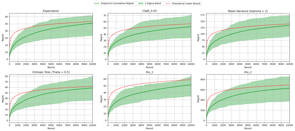
The red curve indicates the theoretical asymptotic lower bound, and each diagram reflects the algorithm running for a fixed $10$ -armed Bernoulli bandit, with different risk functionals, even combinations of them:
- $\rho_1 = 0.5 \cdot \mathrm{CVaR}_{0.05} + 0.5 \cdot \mathrm{ER}_{0.5}$
- $\rho_2(\nu_p) = \rho_{\mathrm{MV}_{2}}(\nu_p) + \exp(2p)$
And for them all, the asymptotic lower bound lies happily in their $1$ -sigma bands. (Yes, each algorithm was averaged across $100$ runs!)

And with that, we are truly done. Happy lunar new year!

—Joel Kindiak, 16 Feb 26, 1131H
February 17, 2026
The Central Limit Theorem

We are now ready to ascend the mountain of proving the central limit theorem, which we will take inspiration from this paper by Calvin Wooyoung Chin.

Lemma 1. Let $X$ be a real-valued random variable with finite expectation. For any $\delta > 0$ ,

$\displaystyle \mathbb P(|X| \geq \delta) \leq \frac{\mathbb E[|X|]}{\delta}.$

This is called Markov’s inequality. Furthermore, if $X$ has finite variance, then

$\displaystyle \mathbb P(|X - \mathbb E[X]| \geq \delta ) \leq \frac{\mathrm{Var}(X)}{\delta^2}.$

This is called Chebychev’s inequality.

Proof. For the first identity,

$\begin{aligned} \mathbb E[|X|] &= \mathbb E[|X| \cdot \mathbb I_{[\delta, \infty)}] + \mathbb E[|X| \cdot \mathbb I_{(-\infty, \delta)}] \\ &\geq \mathbb E[\delta \cdot \mathbb I_{[\delta, \infty)}] + 0\\ &= \delta \cdot \mathbb E[\mathbb I_{[\delta, \infty)} ] \\ &= \delta \cdot \mathbb P(|X| \geq \delta). \end{aligned}$

Dividing by $\delta$ yields the desired result. For Chebychev’s inequality, apply Markov’s inequality to the random variable $(X - \mathbb E[X])^2$ to get

$\begin{aligned} \mathbb P(|X - \mathbb E[X]| \geq \delta) &= \mathbb P( (X - \mathbb E[X])^2 \geq \delta^2 ) \\ &= \frac{\mathbb E[(X - \mathbb E[X])^2]}{\delta^2} \\ &\leq \frac{\mathrm{Var}(X)}{\delta^2}. \end{aligned}$

Chebychev’s inequality is also responsible for our intuition about probability arising from repeated experiments.

Corollary 1. Fix $K \subseteq \Omega$ and denote $p:= \mathbb P(K)$ . Define the i.i.d. random variables $\xi_i$ by $\xi_i = \mathbb I_K$ , so that $\xi_i \sim \mathrm{Ber}(p)$ . Define

$\displaystyle \bar \xi_n := \frac 1n \cdot \sum_{i=1}^n \xi_i.$

Then for any $\delta > 0$ , $\mathbb P(|\bar \xi_n - p| > \delta) \to 0$ . In this case, we say that $\bar \xi_n \to p$ in probability.

Proof. Fix $\delta > 0$ . Since $\mathbb E[\xi_n] = p$ and $\mathrm{Var}(\xi_n) = p(1-p)$ ,

$\displaystyle \mathbb E[\bar \xi_n] = p,\quad \mathrm{Var}(\bar \xi_n) = \frac{p(1-p)}{n}.$

By Chebychev’s inequality,

$\begin{aligned} \mathbb P(|\bar \xi_n - p| > \delta) &\leq \frac{\mathrm{Var}(\bar \xi_n)}{\delta^2} = \frac{p(1-p)}{n \cdot\delta^2}. \end{aligned}$

Taking $n \to \infty$ , $\mathbb P(|\bar \xi_n - p| > \delta) \to 0$ .

Denote $Z \sim \mathcal N(0, 1)$ and its c.d.f. by $\Phi$ .

Lemma 2. Let $X_1, X_2,\dots$ be real-valued random variables. Suppose for any thrice-differentiable $f : \mathbb R \to \mathbb R$ such that $f, f', f'', f'''$ are bounded,

$\displaystyle \lim_{n \to \infty} \mathbb E[f(X_n)] = \mathbb E[f(Z)].$

Then for any $z \in \mathbb R$ ,

$\displaystyle \lim_{n \to \infty} \mathbb P(X_n \leq z) = \Phi(z),\quad z \in \mathbb R.$

Proof. Fix $z \in \mathbb R$ and $\epsilon > 0$ . Since the p.d.f. of $Z$ is continuous, there exists $\delta > 0$ such that

$|\Phi(z \pm \delta) - \Phi(z)| < \epsilon.$

In particular, $\Phi(z+\delta) < \Phi(z) < \Phi(z-\delta) + \epsilon$ . Define thrice-differentiable bounded functions $f, F : \mathbb R \to [0, 1]$ with bounded first, second, and third derivatives such that

$f|_{(-\infty, z-\delta]} = 1,\quad f|_{[z, \infty)} = 0,\quad F|_{(-\infty, z]} = 1,\quad F|_{[z+\delta, \infty)} = 0.$

By hypothesis,

$\displaystyle \lim_{n \to \infty} \mathbb E[f(X_n)] = \mathbb P(Z \leq z -\delta) = \Phi(z-\delta) \geq \Phi(z) - \epsilon.$

Similarly, $\mathbb E[F(X_n)] < \Phi(z) + \epsilon$ . Since $f \leq \mathbb I_{(-\infty, z]} \leq F$ point-wise, for sufficiently large $n$ ,

$\Phi(z) - \epsilon < \mathbb E[f(X_n)] \leq \underbrace{ \mathbb E[ \mathbb I_{(-\infty, z]} ] }_{ \mathbb P(X_n \leq z)} \leq \mathbb E[F(X_n)] < \Phi(z) + \epsilon,$

so that $\displaystyle \lim_{n \to \infty} \mathbb P(X_n \leq z) = \Phi(z)$ , as required.

Theorem 1 (Central Limit Theorem). Let $X_1,X_2,\dots$ be i.i.d. with mean $0$ and variance $1$ . Then for any $z \in \mathbb R$ ,

$\displaystyle \lim_{n \to \infty} \mathbb P(\sqrt n \cdot \bar X_n \leq x) = \Phi(z).$

In this case, we say that $\sqrt n \cdot \bar X_n \to Z$ in distribution.

Proof. Fix i.i.d. $Y_1,Y_2,\dots \sim \mathcal N(0, 1)$ that are independent of $X_1,X_2,\dots$ . For each $n \in \mathbb N$ and $0 \leq i \leq n$ , define

$\displaystyle Z_{n,i} := \frac 1{\sqrt{n}} \cdot \left( \sum_{j=1}^i X_j + \sum_{j=i+1}^n Y_j \right),\quad S_{n,i} := Z_{n,i} - \frac 1{\sqrt{n}} \cdot X_i.$

By direct computations, $Z_{n,n} = \sqrt{n} \cdot \bar X_n$ and $Z_{n,0} = Z \sim \mathcal N(0, 1)$ . The key idea is using Lemma 2 to conclude our proof. Fix any thrice-differentiable $f : \mathbb R \to \mathbb R$ such that $f, f', f'', f'''$ are bounded. We claim that

$\displaystyle \lim_{n \to \infty} \mathbb E[f(Z_{n,n})] = \mathbb E[f(Z_{n,0})].$

Fix $\epsilon > 0$ . We aim to find $N \in \mathbb N$ such that for $n > N$ ,

$\displaystyle |\mathbb E[f(Z_{n,n})] - \mathbb E[f(Z_{n,0})]| < \epsilon.$

Applying Taylor’s theorem for the interval containing $S_{n,i}$ and $Z_{n,i}$ , there exists $C_{n,i}$ between them such that

$\displaystyle f(Z_{n_i}) = f(S_{n,i}) + f'(S_{n,i}) \cdot (Z_{n,i} - S_{n,i}) + \frac{f''(C_{n,i})}{2!} \cdot (Z_{n,i} - S_{n,i})^2.$

Performing algebra yields

$\displaystyle f(Z_{n,i}) - f(S_{n,i}) - f'(S_{n,i}) \cdot \frac{X_i}{\sqrt n} - f''(S_{n,i}) \cdot \frac{X_i^2}{2 n} = \underbrace{ \frac{ ( f''(C_{n,i}) - f''(S_{n,i}) ) X_i^2}{2n} }_{R_{n,i}}.$

Since $f'''$ is bounded, there exists $\delta > 0$ such that

$\delta \cdot \| f''' \|_\infty \leq \epsilon.$

By the mean value theorem, whenever $|x - y| \leq \delta$ ,

$|f''(x) - f''(y)| \leq \| f''' \|_\infty \cdot |x - y| \leq \delta \cdot \| f''' \|_\infty \leq \epsilon.$

Consider the “good event” $G := \{ |X_i| \leq \delta \sqrt{n} \}$ and its complement

$G^c := \Omega \backslash G = \{ |X_i| > \delta \sqrt{n} \}.$

By our bound on the second derivative via the mean value theorem, we can bound $R_{n,i}$ in the “good event” $G$ by

$\displaystyle |f''(C_{n,i}) - f''(S_{n,i})| \leq \epsilon \quad \Rightarrow \quad \mathbb E[|R_{n,i}| \cdot \mathbb I_G] \leq \frac{\epsilon}{2n} \cdot \mathbb E[X_i^2] = \frac{\epsilon}{2n}.$

On the other hand, in the “bad event” $G^c$ , since $\| f'' \|_\infty \leq M$ for some $M > 0$ ,

$\displaystyle \mathbb E[|R_{n,i}| \cdot \mathbb I_{G^c}] \leq \frac{M}{n} \cdot \mathbb E[X_i^2 \cdot \mathbb I_{G^c}] \leq \frac Mn \cdot \mathbb E[\mathbb I_{G^c}].$

By Chebychev’s inequality,

$\begin{aligned}\mathbb E[\mathbb I_{G^c}] &= \mathbb P(|X_i| \geq \delta \sqrt n) \leq \frac{1}{\delta \cdot \sqrt{n}^2} = \frac{1}{n \delta}.\end{aligned}$

Therefore,

$\displaystyle \mathbb E[|R_{n,i}|] = \mathbb E[|R_{n,i}| \cdot \mathbb I_G] + \mathbb E[|R_{n,i}| \cdot \mathbb I_{G^c}] \leq \left( \frac{\epsilon}{2} + \frac{M}{n\delta} \right) \cdot \frac 1n.$

Thus, selecting $N > 2M/(\epsilon \delta)$ yields $\mathbb E[|R_{n,i}|] \leq \epsilon/n$ . Plugging in the left-hand side of $R_{n,i}$ ,

$\displaystyle |\mathbb E[f(Z_{n,i})] - \mathbb E[f(S_{n,i})] - \mathbb E[f''(S_{n,i}) ] / 2n |\leq \frac{\epsilon}{n}.$

The argument remains almost unchanged with $Z_{n,i}$ replaced with $Z_{n,i-1}$ , so that we have the bound

$\displaystyle |\mathbb E[f(Z_{n,i-1})] - \mathbb E[f(S_{n,i})] - \mathbb E[f''(S_{n,i}) ] / 2n |\leq \frac{\epsilon}{n}.$

Applying the triangle inequality,

$\displaystyle |\mathbb E[f(Z_{n,i})] - \mathbb E [f(Z_{n,i-1})]| \leq \frac{\epsilon}{n} + \frac{\epsilon}{n} = \frac{2\epsilon}{n}.$

Finally, applying a telescoping series,

$\begin{aligned} |\mathbb E[f(Z_{n,n})] - \mathbb E [f(Z_{n,0})]| &\leq \sum_{i=1}^n |\mathbb E[f(Z_{n,i})] - \mathbb E [f(Z_{n,i-1})]| \leq \sum_{i=1}^n \frac{2\epsilon}n = 2\epsilon. \end{aligned}$

Replace $\epsilon$ with $\epsilon/3$ to complete the argument.

With that, we are done with probability…for now. There are many directions we can take from this point on. We could have proven this result using techniques involving characteristic functions or even Brownian motion, but those topics will require their entire blog sections in order to properly discuss. We conclude with the famous normal approximation to the binomial and Poisson distributions.

Corollary 1. For $X_n \sim \mathrm{Bin}(n, p)$ ,

$\displaystyle \lim_{n \to \infty} \mathbb P \left( \frac{X_n - np}{\sqrt{np(1-p)}} \leq z \right) = \Phi(z).$

This is the normal approximation to the binomial distribution.

Proof. For each $n$ , write $X_n := \sum_{i=1}^n \xi_i$ for i.i.d. $\xi_i \sim \mathrm{Ber}(p)$ and

$\displaystyle Y_n := \frac{ X_n - np }{ \sqrt{p(1-p)} } .$

Then

$\displaystyle \bar Y_n := \frac 1n \cdot Y_n = \frac 1n \cdot \sum_{i=1}^n \frac{ \xi_i - p }{\sqrt{p(1-p)}} = \frac{X_n - np}{n \sqrt{p(1-p)}}.$

Since the $(\xi_i - p)/\sqrt{p(1-p)}$ are i.i.d. with mean $0$ and variance $1$ , by the central limit theorem,

$\displaystyle \lim_{n \to \infty} \mathbb P \left( \frac{X_n - np}{\sqrt{np(1-p)}} \leq z \right) = \lim_{n \to \infty} \mathbb P ( \sqrt n \cdot \bar Y_n \leq z) = \Phi(z).$

Corollary 2. We have

$\displaystyle \lim_{\lambda \to \infty} \mathbb P \left( \frac{X - \lambda}{\sqrt{\lambda}} \leq z \right) = \Phi(z), \quad X \sim \mathrm{Pois}(\lambda).$

This is the normal approximation to the Poisson distribution.

Proof. Assume $\lambda \in \mathbb N^+$ . Write $X_{\lambda} := \sum_{i=1}^{\lambda} \xi_i$ for i.i.d. $\xi_i \sim \mathrm{Pois}(1)$ and

$\displaystyle Y_\lambda := X_{\lambda} - \lambda .$

Then

$\displaystyle \bar Y_{\lambda} = \frac{X_{\lambda} - \lambda}{\lambda } = \frac 1{\lambda} \cdot \sum_{i=1}^{\lambda} (\xi_i - 1).$

Since the $\xi_i - 1$ are i.i.d. with mean $0$ and variance $1$ , by the central limit theorem,

$\displaystyle \lim_{\lambda \to \infty} \mathbb P \left( \frac{X_{\lambda} - \lambda}{ \sqrt{\lambda} } \leq z \right) = \lim_{n \to \infty} \mathbb P ( \sqrt{ \lambda } \cdot \bar Y_\lambda \leq z) = \Phi(z).$

—Joel Kindiak, 31 Jul 25, 1359H

December 9, 2025
Adding Random Variables…Revisited

We are now justified in adding random variables. For instance, if $X, Y \sim \mathcal N(0, 1)$ , what is the distribution of $X + Y$ ? Unfortunately, in the most extreme cases, this answer is trivial.

Lemma 1. Let $X \sim \mathcal N(0, 1)$ and $Y = -X$ . Then $Y \sim \mathcal N(0, 1)$ and $X + Y = 0$ .

Proof. We observe that for any $K \in \frak{B}(\mathbb R)$ , since $f_X(\cdot) = f_X(-\cdot)$ , by a change of variables,

$\begin{aligned} \mathbb P_Y(K) = \mathbb P_X(-K) &= \int_{-K} f_X(x)\, \mathrm dx \\ &= \int_K f_X(-x)\, \mathrm dx \\ &= \int_K f_X(x)\, \mathrm dx = \mathbb P_X(K).\end{aligned}$

Therefore, for any $K \in \frak{B}(\mathbb R)$ ,

$\displaystyle \int_K f_Y\, \mathrm d\lambda = \int_K f_X\, \mathrm d\lambda.$

Therefore, $f_Y = f_X$ so that $Y \sim \mathcal N(0, 1)$ .

Here, it is clear that $Y$ is entirely dependent— $100\%$ correlated even—to the random variable $X$ . We got a rather useless answer to our question in this case. If instead we swung to the other extreme, namely $X,Y$ being independent, we don’t have a general formula for any $X, Y$ . Nevertheless, the independent case proves to be far more useful in reality—for instance, the exam scores of two students are effectively independent barring (sufficiently drastic) externalities.

Therefore, let’s discuss what it means for two random variables $X,Y : \Omega \to \mathbb R$ to be independent. We have previously seen that two events $K,L$ are called independent if $\mathbb P(K \cap L) = \mathbb P(K) \cdot \mathbb P(L)$ .

Lemma 2. The set $\sigma(X) := \{X^{-1}(K) : K \in \frak{B}(\mathbb R)\} \subseteq \mathcal F$ forms a $\sigma$ -algebra, called the $\sigma$ -algebra generated by $X$ .

Given two $\sigma$ -algebras $\mathcal F_1, \mathcal F_2 \subseteq \mathcal F$ , also known as sub- $\sigma$ -algebras of $\mathcal F$ , we say that $\mathcal F_1, \mathcal F_2$ are independent if for any $K \in \mathcal F_1, L \in \mathcal F_2$ , $K, L$ are independent.

Definition 1. Two random variables $X, Y$ are said to be independent if $\sigma(X), \sigma(Y)$ are independent.

Suppose $\mathbb P_X \ll \mu$ and $\mathbb P_Y \ll \mu$ , where $\mu$ denotes either the counting measure $|\cdot|$ or the Lebesgue measure $\lambda$ . Let $\mu^2$ be the product of two copies of $\mu$ . Suppose $(X,Y) \ll \mu^2$ .

Theorem 1. $X, Y$ are independent and $(X,Y) \ll \mu^2$ if and only if

$\displaystyle \mathbb P((X, Y) \in K) = \int_K f_X \cdot f_Y\, \mathrm d\mu^2,$

where the integrand in the right-hand side is interpreted to mean

$f_X(\cdot , y) = f_X,\quad f_Y(x, \cdot) = f_Y, \quad x, y \in \mathbb R.$

Proof. Consider the cumulative distribution functions

$F_X(x) := \mathbb P(X \in (-\infty, x]) \equiv \mathbb P(X \leq x),\quad F_Y(y) := \mathbb P( Y \leq y).$

By the Radon-Nikodým theorem,

$\displaystyle F_X(x) = \int_{(-\infty, x]} f_X\, \mathrm d\mu,\quad F_Y(y) = \int_{(-\infty, y]} f_Y\, \mathrm d\mu.$

In the direction $(\Leftarrow)$ , by the Fubini-Tonelli theorem,

$\begin{aligned} \mathbb P(X^{-1}((-\infty, x]) \cap Y^{-1}((-\infty, y])) &= \mathbb P((X,Y) \in (-\infty, x] \times (-\infty, y]) \\ &= \int_{(-\infty, x] \times (-\infty, y]} f_{X,Y}\, \mathrm d\mu^2 \\ &= \int_{(-\infty, x]} \int_{(-\infty, y]} f_{X,Y}\, \mathrm d \mu\, \mathrm d \mu \\ &= \int_{(-\infty, x]} \int_{(-\infty, y]} f_X \cdot f_Y\, \mathrm d \mu\, \mathrm d \mu \\ &= \int_{(-\infty, x]} f_X \, \mathrm d \mu \cdot \int_{(-\infty, y]} f_Y\, \mathrm d \mu \\ &= \mathbb P(X^{-1}(-\infty, x]) \cdot \mathbb P(Y^{-1}(-\infty, y]), \end{aligned}$

establishing independence.

In the direction $(\Rightarrow)$ , we similarly use the Fubini-Tonelli theorem to obtain

$\begin{aligned} \iint_{(-\infty, x] \times (-\infty, y]} f_{X,Y}\, \mathrm d\mu^2 &= \int_{(-\infty, x]} f_X\, \mathrm d\mu \cdot \int_{(-\infty, y]} f_Y\, \mathrm d\mu \\ &= \int_{(-\infty, x]} \int_{(-\infty, y]} f_X \cdot f_Y\, \mathrm d \mu\, \mathrm d \mu \\ &= \iint_{(-\infty, x] \times (-\infty, y]} f_X \cdot f_Y\, \mathrm d\mu^2, \end{aligned}$

so that $f_{X,Y} = f_X \cdot f_Y$ .

Henceforth, when $X,Y$ are independent and $X \ll \mu$ and $Y \ll \mu$ , we assume $(X,Y) \ll \mu$ so that $f_{X,Y}$ is a meaningful quantity.

Corollary 1. Define

$\displaystyle F_{X,Y}(x,y) = \mathbb P((X,Y) \in (-\infty, x] \times (-\infty, y]) \equiv \mathbb P(X \leq x, Y \leq y).$

Then $X, Y$ are independent and $(X,Y) \ll \mu^2$ if and only if for any $x, y \in \mathbb R$ ,

$\displaystyle F_{X,Y}(x,y) = F_X(x)\cdot F_Y(y).$

Finally, let’s add these random variables together.

Theorem 1. If $X, Y$ are independent $\mathbb R$ -valued random variables with density functions $f_X, f_Y$ , then $X+Y$ is a random variable with density function

$f_{X+Y} = f_X * f_Y,$

where the right-hand side denotes convolution with respect to $\mu$ :

$\displaystyle (f * g)(u) := \int_{\mathbb R} f \cdot g(u- \cdot )\, \mathrm d\mu \equiv \int_{\mathbb R} f(x) \cdot g(u- x )\, \mathrm d\mu(x).$

If $\mu$ is the counting measure, we get

$\displaystyle (f * g)(u) = \sum_{n \in \mathbb Z} f(n) \cdot g(u-n).$

If $\mu$ is the Lebesgue measure, we get

$\displaystyle (f * g)(u) = \int_{-\infty}^{\infty} f(t) \cdot g(u-t)\, \mathrm dt.$

Proof. Denote $g(x,y) = x+y$ so that for any fixed $x$ , $g(x,y) \leq u$ if and only if $y \leq u - x$ . For any $K \in \frak{B}(\mathbb R)$ ,

$\displaystyle \begin{aligned} \int_{K} f_{X+Y}\, \mathrm d\mu &= \mathbb P(X+Y \in K) \\ &= \mathbb P((X,Y) \in g^{-1}(K)) \\ &= \int_{g^{-1}(K)} f_{X,Y}\, \mathrm d\mu^2 \\ &= \int_{g^{-1}(K)} f_{X,Y}(x,y)\, \mathrm d\mu^2(x,y) \\ &= \int_{\mathbb R} \int_{K-x} f_{X,Y}(x,y)\, \mathrm d\mu(y)\, \mathrm d\mu(x) \\ &= \int_{\mathbb R} \int_{K} f_{X,Y}(x,y-x)\, \mathrm d\mu(y)\, \mathrm d\mu(x) \\ &= \int_{K} \int_{\mathbb R} f_{X,Y}(x,y-x)\, \mathrm d\mu(x)\, \mathrm d\mu(y) \\ &= \int_{K} \underbrace{ \int_{\mathbb R} f_{X}(x) \cdot f_Y(y-x)\, \mathrm d\mu(x) }_{(f_X * f_Y)(y)} \, \mathrm d\mu(y) = \int_{K} f_X * f_Y\, \mathrm d\mu. \end{aligned}$

Finally, let’s concretely add two independently normally distributed random variables.

Theorem 2. If $X \sim \mathcal N(\mu_1, \sigma_1^2)$ and $Y \sim \mathcal N(\mu_2, \sigma_2^2)$ are independent, then $X + Y \sim \mathcal N(\mu_1 + \mu_2, \sigma_1^2 + \sigma_2^2)$ .

Proof. Write $X = \mu_1 + \sigma_1 Z_1$ and $Y = \mu_2 + \sigma_2 Z_2$ . Then

$X + Y = (\mu_1 + \mu_2) + \sigma_1 Z_1 + \sigma_2 Z_2,$

where $Z_1, Z_2 \sim \mathcal N(0, 1)$ are independent. It suffices to prove that

$\sigma_1 Z_1 + \sigma_2 Z_2 \sim \mathcal N(0, \sigma_1^2 + \sigma_2^2).$

By construction, for any $\sigma > 0$ , if $U \sim \mathcal N(0, \sigma^2)$ , then

$\displaystyle f_U(u) = \frac{1}{ \sigma \sqrt{2\pi} } e^{-\frac{u^2}{2\sigma^2} }.$

Defining $W := \sigma_1 Z_1 + \sigma_2 Z_2$ ,

$\begin{aligned} f_W(w) &= (f_{\sigma_1 Z_1} * f_{\sigma_2 Z_2})(w) \\ &= \int_{-\infty}^{\infty} \frac{1}{ \sigma_1 \sqrt{2\pi} } e^{-\frac{t^2}{2\sigma_1^2} } \cdot \frac{1}{ \sigma_2 \sqrt{2\pi} } e^{-\frac{(w-t)^2}{2\sigma_2^2} }\, \mathrm dt \\ &= \frac{1}{\sigma_1 \sigma_2 \cdot 2\pi}\int_{-\infty}^{\infty} \exp\left( - \frac 12 \left( \frac{t^2}{\sigma_1^2} + \frac{(w-t)^2}{\sigma_2^2} \right)\right)\, \mathrm dt. \end{aligned}$

By algebruh,

$\displaystyle \frac{t^2}{\sigma_1^2} + \frac{(w-t)^2}{\sigma_2^2} = \left( \frac{1}{\sigma_1^2} + \frac{1}{\sigma_2^2} \right) t^2 - \frac{2w}{\sigma_2^2} \cdot t + \frac{w^2}{\sigma_2^2} = A(t - h)^2 + k.$

for carefully calculated constants $A, h, k$ , in particular, with

$\displaystyle A = \frac{1}{\sigma_1^2} + \frac{1}{\sigma_2^2},\quad k = \frac{w}{A \sigma_2^2} = -\frac 14 \cdot \frac{4w^2}{\sigma_2^4} \cdot \frac{\sigma_1^2 \cdot \sigma_2^2}{\sigma_1^2 + \sigma_2^2} + \frac{w^2}{\sigma_2^2} = -\frac{w^2}{\sigma_1^2 + \sigma_2^2}.$

Denoting $\sigma_3^2 := 1/A$ , the integral then simplifies to

$\begin{aligned}\int_{-\infty}^{\infty} e^{-\frac 12 (A(t-h)^2 + k)}\, \mathrm dt &= e^{-\frac 12 k} \cdot \sigma_3 \cdot \sqrt{2\pi} \cdot \underbrace{ \int_{-\infty}^{\infty} \frac{1}{\sigma_3 \sqrt{2\pi} }e^{-\frac {(t-h)^2}{2\sigma_3^2}} \, \mathrm dt }_1 \\ &= e^{-\frac 12 k} \cdot \sigma_3 \cdot \sqrt{2\pi}.\end{aligned}$

Therefore, denoting $\sigma^2 := \sigma_1^2 + \sigma_2^2$ so that $k = -w^2/\sigma^2$ ,

$\begin{aligned} f_W(w) &= \frac{\sigma_3}{\sigma_1 \sigma_2} \cdot \frac{1}{\sqrt{2\pi}} \cdot e^{-\frac 12 k} = \frac{1}{\sigma \sqrt{2\pi}} e^{-\frac{w^2}{2\sigma^2}}. \end{aligned}$

Therefore, $\sigma_1 Z_1 + \sigma_2 Z_2 = W \sim \mathcal N(0, \sigma^2) = \mathcal N(0, \sigma_1^2 + \sigma_2^2)$ , as required.

In practice, to compute probabilities involving normal distributions, we define

$\displaystyle \Phi(z) := \mathbb P(Z \leq z) = \frac 12 + \frac{1}{\sqrt{2\pi}} \int_0^z e^{-t^2/2}\, \mathrm dt$

and tabulate commonly used approximate values of $\Phi(z)$ for $z > 0$ , known in the statistics community as a $z$ -table. By symmetry, $\Phi(-z) = 1- \Phi(z)$ . For any $X \sim \mathcal N(\mu, \sigma^2)$ , since $X = \mu + \sigma Z$ , we can reduce the computation to

$\displaystyle \mathbb P(X \leq x) = \mathbb P\left( Z \leq \frac{x - \mu}{\sigma} \right) = \Phi \left( \frac{x - \mu}{\sigma}\right).$

By induction, we have the following sampling distribution $\bar X_n$ .

Corollary 2. For independent, identically distributed random variables $X_1,\dots, X_n \sim \mathcal N(\mu, \sigma^2)$ ,

$\displaystyle \bar X_n := \frac{1}{n} \sum_{i=1}^n X_i \sim \mathcal N \left( \mu, \frac{\sigma^2}{n} \right).$

The central limit theorem claims that even if $X_i$ are not normally distributed, $\bar X_n$ converges in distribution to $\mathcal N(\mu, \sigma^2/n)$ . For the limiting distribution to be constant, the equivalent claim is that $(\bar X_n-\mu) / (\sigma / \sqrt{n})$ converges in distribution to $Z \sim \mathcal N(0, 1)$ .

We have previously stated the special case $(\mu, \sigma) = (0, 1)$ and aim to prove it properly using techniques in stochastic calculus. If we have this result, we are emboldened to carry out hypothesis tests, which are commonplace in the STEM fields as well as the data-driven social sciences. We will digress to this application before we dive right back into our ascent toward the central limit theorem.

—Joel Kindiak, 23 Jul 25, 2257H

December 5, 2025
Legitimate Integral Swapping

Given two random variables $X, Y$ , what is the distribution of $X + Y$ ? We could define the discrete random variables, and perhaps continuous ones as well. But let’s go back to measure theory and define the joint distribution $(X, Y)$ as rigorously as possible.

Let $(\Omega, \mathcal F, \mu)$ be a measure space (or a probability space if $\mu$ is a probability measure). Equip $\mathbb R^n$ is equipped with the Borel $\sigma$ -algebra $\frak{B}(\mathbb R^n)$ , generated by open balls under the Euclidean metric.

Lemma 1. Let $X, Y : \Omega \to \mathbb R$ be a random variable. Then $(X,Y) : \Omega \to \mathbb R^2$ defined by $(X,Y)(\omega) := (X(\omega), Y(\omega))$ is a random variable.

Proof. The map $(X,Y)$ is continuous, and therefore, has open sets as pre-images of open sets. Therefore, $(X,Y)$ is $\mathcal F$ / $\frak{B}(\mathbb R^2)$ -measurable.

What would be a reasonable measure on $\mathbb R^2$ ? Intuitively, we should have a measure $\lambda_2$ on $\mathbb R^2$ such that $\lambda_2(K \times L) = \lambda_1(K) \cdot \lambda_1(L)$ , where $\lambda_1$ denotes the usual Lebesgue measure that we painstakingly constructed. In fact, more generally, given measure spaces $(\Omega_i, \mathcal F_i, \mu_i)$ , we would like to define a reasonable $\sigma$ -algebra $\mathcal F$ on $\Omega := \prod_{i=1}^n \Omega_i$ and a measure $\mu$ on $\mathcal F$ such that

$\displaystyle \mu\left( \prod_{i=1}^n K_i \right) = \prod_{i=1}^n \mu_i(K_i),\quad K_i \in \mathcal F_i.$

It turns out that with the help of Carathéodory’s extension theorem, this task isn’t as Sisyphean as it seems.

Theorem 1. Given measure spaces $(\Omega_i, \mathcal F_i, \mu_i)$ , there exists a $\sigma$ -algebra $\mathcal F$ on $\Omega := \prod_{i=1}^n \Omega_i$ and a measure $\mu$ on $\mathcal F$ such that $\prod_{i=1}^n K_i \in \mathcal F$ and

$\displaystyle \mu\left( \prod_{i=1}^n K_i \right) = \prod_{i=1}^n \mu_i(K_i),\quad K_i \in \mathcal F_i.$

Proof. We will prove the special case $n = 2$ for simplicity. Define the algebra

$\mathcal F^0 := \{ K \times L : K \in \mathcal F_1, L \in \mathcal F_2\}.$

For any $K \in \mathcal F_1$ and $x \in \Omega_1$ , define the $x$ -section $K_x \subseteq \Omega_2$ by

$K_x := \{ y \in \Omega_2 : (x, y) \in K\}.$

Define the $y$ -section $K^y$ similarly. Now given $M := \bigcup_{i=1}^n K_i \times L_i \in \mathcal F^0$ , for any $x \in \Omega_1$

$\displaystyle M_x = \bigcup_{i : x \in K_i} L_i \in \mathcal F_2.$

Therefore, the quantity $\mu_2(M_x)$ is well-defined. Similarly, $\mu_1(M^y)$ is well-defined for any $y \in \Omega_2$ . Hence, define the function $f_M(x) := \mu_2(M_x)$ , which is non-negative and simple since in the special case $M = (K_1 \times L_1) \cup (K_2 \times L_2)$ ,

$f_M = \mu_2(L_1 \cup L_2) \cdot \mathbb I_{K_1 \cap K_2} + \mu_2(L_1) \cdot \mathbb I_{K_1 \backslash K_2} + \mu_2(L_2) \cdot \mathbb I_{K_2 \backslash K_1}.$

We can similarly define $g_M(y) := \mu_1(M^y)$ , and define

$\displaystyle \mu_0(M) := \int_{\Omega_1} f_M\, \mathrm d\mu_1 = \int_{\Omega_2} g_M\, \mathrm d\mu_2.$

To see this in the simplest case when $M$ is a disjoint union (the rest follows by careful bookkeeping),

$\displaystyle \int_{\Omega_1} f_M\, \mathrm d\mu_1 = \sum_{i=1}^n \mu_2(L_i) \cdot \mu_1(K_i) = \int_{\Omega_2} g_M\, \mathrm d\mu_2.$

In particular, $\mu_0(K \times L) = \mu_1(K) \cdot \mu_2(L)$ . We claim that $\mu_0$ is countably additive. Fix $M = \bigsqcup_{i=1}^\infty M_i \in \mathcal F^0$ . Then for any $x \in \Omega_1$ ,

$\displaystyle f_M(x) = \mu_2(M_x) = \mu_2 \left( \bigsqcup_{i=1}^\infty (M_i)_x \right) = \sum_{i=1}^\infty \mu_2((M_i)_x) = \sum_{i=1}^\infty f_{M_i}(x).$

Therefore, the function $\sum_{i=1}^n f_{M_i}$ converges monotonically to $f_M$ , and by the monotone convergence theorem,

$\displaystyle \mu_0(M) = \int_{\Omega_1} f_M\, \mathrm d\mu_1 = \sum_{i=1}^\infty \int_{\Omega_1} f_{M_i}\, \mathrm d\mu_1 = \sum_{i=1}^\infty \mu_0(M_i).$

Now apply Carathéodory’s extension theorem to obtain a $\sigma$ -algebra $\mathcal F \supseteq \mathcal F^0$ and a measure $\mu : \mathcal F \to [0, \infty]$ such that $\mu|_{\mathcal F^0} = \mu_0$ .

Theoretically, we could just start defining random variables on the product space $\Omega_1 \times \Omega_2$ and go on our merry way. But we still need to answer a key question: given the distributions $\mathbb P_X$ and $\mathbb P_Y$ , how do we compute $\mathbb P_{X+Y}$ ? In a more abstract manner, we need to integrate with respect to our newly minted measure $\mu$ in a computationally consistent manner with integrals with respect to our old measures $\mu_1,\mu_2$ respectively. Surprisingly, answering this question leads us to one of the most important theorems in multivariable calculus, which is Fubini’s theorem, as it allows us to rigorously swap integrals—a key tool in any reasonable calculation.

Denote the base measure spaces by $\Omega_1 \equiv (\Omega_1,\mathcal F_1,\mu_1)$ and $\Omega_2 \equiv (\Omega_2,\mathcal F_2,\mu_2)$ , and their product space by $\Omega \equiv (\Omega, \mathcal F, \mu)$ . By construction, $\mathcal F \supseteq \mathcal F_1 \times \mathcal F_2$ . We remark that for any $M \in \mathcal F_1 \times \mathcal F_2$ and $x \in \Omega_1, y \in \Omega_2$ , $M_x \in \mathcal F_2$ and $M^y \in \mathcal F_1$ , since the $\sigma$ -algebra

$\{M \in \mathcal F : \forall x \in \Omega_1\ \forall y \in \Omega_2\ M_x \in \mathcal F_1 \wedge M^y \in \mathcal F_2\}$

contains $\mathcal F_1 \times \mathcal F_2$ .

Now we observe that $\mathbb R = \bigcup_{n \in \mathbb Z} [n, n+1)$ and each $[n, n+1)$ has Lebesgue measure $1$ .

Definition 1. A measure space $(\Omega, \mathcal F, \mu)$ is $\sigma$ -finite if there exist $K_1,K_2\dots$ with $\mu(K_i) < \infty$ such that $\Omega = \bigcup_{i=1}^\infty K_i$ . For instance, $\mathbb R^n$ is $\sigma$ -finite.

Lemma 2. Suppose $\Omega_1,\Omega_2$ are $\sigma$ -finite. For any $M \in \mathcal F_1 \times \mathcal F_2$ , the non-negative functions $f_M(x) := \mu_2(M_x)$ and $g_M(y) := \mu_1(M^y)$ are measurable, and define the predicate $\phi$ by

$\displaystyle \phi(M) := \left( \int_{\Omega_1} f_M\, \mathrm d\mu_1 = \mu(M) = \int_{\Omega_2} g_M\, \mathrm d\mu_2 \right).$

Then $\phi(M)$ holds for any $M \in \mathcal F_1 \times \mathcal F_2$ . Note that this result is an extension from that of Theorem 1.

Proof. We first prove the case that $\mu_1(\Omega_1) < \infty$ and $\mu_2(\Omega_2) < \infty$ . It is straightforward that $\phi(M)$ holds if $M \in \mathcal F^0$ or even a disjoint union of sets in $\mathcal F^0$ . If $\phi(M_1)$ and $\phi(M_2)$ , then $\phi(M_1 \backslash M_2)$ . Finally, if $M_1 \subseteq M_2 \subseteq \dots$ and $\phi(M_i)$ , then defining $M = \bigcup_{i=1}^\infty M_i$ , $f_M = \lim_{n \to\infty} f_{M_n}$ is measurable, and by the monotone convergence theorem,

$\displaystyle \int_{\Omega_1} f_M\, \mathrm d\mu_1 = \lim_{n \to \infty} \int_{\Omega_1} f_{M_n}\, \mathrm d\mu_1 = \lim_{n \to \infty} \mu(M_n) = \mu(M).$

Therefore, $\phi(M)$ . Let $\mathcal F' \supseteq \mathcal F_0$ denote the smallest subset of $\mathcal F$ such that these two properties are satisfied. We can verify that $\mathcal F'$ is a $\sigma$ -algebra, and hence contains $\mathcal F_1 \times \mathcal F_2$ , as required.

We now generalise to the $\sigma$ -finite case. Suppose $K_1 \subseteq K_2 \subseteq \dots$ such that $\bigcup_{i=1}^\infty K_i = \Omega_1$ , and $\bigcup_{i=1}^\infty L_i = \Omega_2$ similarly. For each $I$ , define $M_i := M \cap (K_i \times L_i)$ so that $M = \bigcup_{i=1}^\infty M_i$ . The result follows by the monotone convergence theorem.

Lemma 3. For any map $f : \Omega_1 \times \Omega_2 \to [0, \infty]$ , all of its sections

$f_x := f(x, \cdot) : \Omega_2 \to [0, \infty],\quad f^y := f( \cdot, y) : \Omega_1 \to [0, \infty]$

are measurable.

Proof. Apply Lemma 2 to the result $f_x^{-1}([a, \infty]) = (f^{-1}([a, \infty]))_x \in \mathcal F_2$ .

We can now discuss the Fubini-Tonelli theorem. The Fubini theorem is the special case when all integrals therein are finite. Here, a function $f : \Omega \to [-\infty, \infty]$ is integrable if $K := f^{-1}(\{-\infty, \infty\})$ has measure zero and $f \cdot \mathbb I_{\Omega \backslash K}$ is integrable.

Theorem 2 (Fubini-Tonelli Theorem). Suppose $\Omega_1,\Omega_2$ are $\sigma$ -finite. If $f:\Omega_1 \times \Omega_2 \to [-\infty, \infty]$ is either non-negative and measurable (resp. integrable), then the functions $g, h$ defined by

$\displaystyle g(x) := \int_{\Omega_2} f(x, \cdot)\, \mathrm d\mu_2,\quad h(y) := \int_{\Omega_1} f(\cdot, y)\, \mathrm d\mu_1$

are measurable (resp. integrable) and

$\displaystyle \int_{\Omega_1} \int_{\Omega_2} f\, \mathrm d\mu_2\, \mathrm d\mu_1 = \int_{\Omega_2} \int_{\Omega_1} f\, \mathrm d\mu_1\, \mathrm d\mu_2 = \int_{\Omega} f\, \mathrm d\mu.$

Proof. We return to the usual simple $\Rightarrow$ non-negative measurable $\Rightarrow$ integrable strategy. If $f = \mathbb I_M$ , then we obtain this result by Lemma 2. The result extends by linearity to non-negative simple functions.

If $f$ is non-negative, find a sequence of non-negative simple functions $\Phi_n$ that monotonically converge to $f$ . By the monotone convergence theorem,

$\displaystyle \int_{\Omega} f\, \mathrm d\mu = \lim_{n \to \infty} \int_{\Omega} \Phi_n\, \mathrm d\mu.$

For each $n$ , define $\varphi_n$ by setting for each $x \in \Omega_1$ , $\varphi_n(x) := \int_{\Omega_2} \Phi_n(x,\cdot)\, \mathrm d\mu_2$ . Then $\varphi_n$ monotonically increases to $g$ . By the monotone convergence theorem again, since $\Phi_n$ are all step functions,

$\displaystyle \int_{\Omega_1} g\, \mathrm d\mu_1 = \lim_{n \to \infty} \int_{\Omega_1} \varphi_n\, \mathrm d \mu_1 = \lim_{n \to \infty} \int_{\Omega} \Phi_n\, \mathrm d\mu = \int_{\Omega} f\, \mathrm d\mu.$

Finally, in the case $f$ is integrable, write $f = f^+ - f^-$ and perform needful bookkeeping.

As much as we feel somewhat justified to add distributions in general, there is one more measure-theoretic machinery we need to discuss—the technical density function known as the Radon-Nikodým derivative. In doing so, we can be justified in letting $f_X$ denote the density function for any sufficiently nice random variable $X$ .

—Joel Kindiak, 21 Jul 25, 2313H

December 2, 2025
Density Functions on Steroids

We have seen that a random variable $X$ is said to be (absolutely) continuous if there exists a continuous, non-negative, integrable function $f_X$ such that for any Borel-measurable $K$ ,

$\displaystyle \mathbb P_X(K) = \int_K f_X\, \mathrm d\lambda.$

In this case, $\mathbb P_X \ll \lambda$ in the sense that for any Borel-measurable $L$ ,

$\lambda(L) = 0 \quad \Rightarrow \quad \mathbb P_X(L) = 0.$

It turns out that the reverse is true.

Theorem 1 (Radon-Nikodým Theorem). Let $(\Omega, \mathcal F)$ be a measurable space. If $\mu, \nu$ are $\sigma$ -finite measures on $(\Omega, \mathcal F)$ such that $\nu \ll \mu$ , then there exists a measurable function $f : \Omega \to [0, \infty]$ such that

$\displaystyle \nu(K) = \int_K f\, \mathrm d\mu.$

Furthermore, $f$ is unique $\mu$ -a.e., called the Radon-Nikodým derivative, denoted $\displaystyle \frac{\mathrm d \nu}{\mathrm d\mu}$ .

In particular, for any measure $\mathbb P_X$ on $(\mathbb R^n, \frak{B}(\mathbb R^n), \lambda)$ , where $\lambda$ denotes the $n$ -dimensional Lebesgue measure,

$\displaystyle f_X := \frac{\mathrm d\mathbb P_X}{\mathrm d\lambda} \quad \iff \quad \mathrm d\mathbb P_X \equiv f_X\, \mathrm d\lambda$

is called the probability density function of $X$ , where the right-hand side follows a legitimate abuse of notation.

Our goal in this post is to prove the Radon-Nikodým theorem. To achieve that goal, we will need to introduce the notion of a signed measure, and a lemma known as Hahn’s decomposition theorem.

Let $(\Omega, \mathcal F)$ be a measurable space.

Definition 1. The map $\mu : \mathcal F \to \mathbb R$ (excluding infinities) is called a signed measure if $\mu(\emptyset) = 0$ and $\mu$ is countably additive.

Theorem 2 (Hahn Decomposition Theorem). If $\mu$ is a signed measure on $(\Omega, \mathcal F)$ , then there exist disjoint measurable sets $P, N \in \mathcal F$ such that

$\displaystyle \mu( \cdot \cap P) \in [0,\infty),\quad \mu( \cdot \cap N) \in (-\infty, 0],\quad P \sqcup N = \Omega.$

In this case, we call the set $P$ a positive set, denoted $P \geq 0$ , and $N$ a negative set, denoted $N \leq 0$ . A set $M$ is null if it is positive and negative, i.e. $\mu( \cdot \cap M) \in \{0\}$ .

Proof of Theorem 2. We first check that $\alpha := \sup \{\mu(K) : K \geq 0\} < \infty$ . If not, then for any $n \in \mathbb N^+$ , there exists $K_n \in \mathcal F$ with $K_n \geq 0$ such that $\mu(K_n) \geq n$ . Then $K := \bigcup_{n=1}^\infty K_n$ has measure $\mu(K) \geq n$ for any $n$ , leading to $\mu(K) = \infty$ , a contradiction.

Therefore, for any $n \in \mathbb N^+$ , there exists $P_n \geq 0$ such that $\alpha - 1/n < \mu(P_n) \leq \alpha$ . It follows by bookkeeping that $P := \bigcup_{n=1}^\infty P_n$ is positive. We claim that $N:= \Omega \backslash P$ is negative.

Suppose otherwise. Then there exists $K \in \mathcal F$ such that $\mu(K \cap N) > 0$ . Assume $K \subseteq N$ so that $\mu(K) > 0$ . If $K$ is positive, then so is $P \cup K$ , thus $\mu(P \cup K) = \mu(P) + \mu(K) > \alpha$ , a contradiction. Therefore, there exists $K_1 \subseteq K$ such that $\mu(K_1) = \mu(K_1 \cap K) < 0$ . Furthermore, $\mu(K \backslash K_1) = \mu(K) - \mu(K_1) > 0$ .

Define $n_1 := \min \{k \in \mathbb N : \mu(K_1) < -1/k\}$ , which exists by the Archimedean property of $\mathbb R$ . Repeating the argument inductively on the set $K \backslash \bigcup_{j=1}^{i-1} K_j$ , we obtain $K \supseteq K_1 \supseteq K_2 \supseteq \dots$ such that $K_i \subseteq K \backslash \bigcup_{j=1}^{i-1} K_j$ and $\mu(K_i) < -1/{n_i}$ , where $n_i$ is the smallest possible positive integer. Define $L := K \backslash \bigsqcup_{i=1}^\infty K_i$ , which has positive finite measure. Since $\mu$ is countably additive,

$\displaystyle \mu(K) = \mu(L) + \sum_{i=1}^\infty \mu(K_i).$

Hence, $\mu(K_i) \to 0 \iff 1/n_i \to 0$ as $i \to \infty$ .

If we can show that $L \geq 0$ , then $\mu(L \cup P) > \alpha$ , yielding the desired contradiction. To that end, suppose for a contradiction that there exists $M \subseteq L$ such that $\mu(M) = \mu(M \cap L) < 0$ . Then $\mu(M) < -1/(n_i - 1)$ for some $n_i$ , contradicting the construction of $K_i$ , as required.

Now we prove the Radon-Nikodým theorem.

Proof of Theorem 1. We first assume that $\mu, \nu$ are finite. For any $n, k$ , define the signed measure $\lambda_{n,k} := \nu - \frac{k}{2^n} \cdot \mu : \mathcal F \to \mathbb R$ . By the Hahn decomposition theorem, there exist disjoint positive and negative sets $P_{n,k}, N_{n,k}$ with respect to $\lambda_{n,k}$ such that $P_{n,k} \sqcup N_{n,k} = \Omega$ .

Since $k\cdot 2^{-n} \geq l \cdot 2^{-m}$ implies $P_{n,k} \subseteq P_{m,l}$ , for any $n$ , $( P_{n,k} )$ is decreasing in $k$ . Define the set $P_n := \bigcap_{k=1}^\infty P_{n,k}$ , which is positive with respect to all $\lambda_{n,k}$ . Since this set is positive with respect to $\lambda_{n,k}$ ,

$\displaystyle \lambda_{n,k}(P_{n,k}) \geq 0 \quad \Rightarrow \quad \mu(P_n) \leq \mu(P_{n,k}) \leq \frac{2^n}{k} \cdot \nu(P_{n,k}) \leq \frac{2^n}{k} \cdot \nu(\Omega).$

Taking $k \to \infty$ , we obtain $\mu(P_n) = 0$ for any $n$ . Define the simple functions

$\begin{aligned} f_{n}^- &:= \sum_{k=1}^\infty \frac{k}{2^n} \cdot \mathbb I_{P_{n,k} \backslash P_{n,k+1}} + \infty \cdot \mathbb I_{P_n}, \\ f_{n}^+ &:= \sum_{k=1}^\infty \frac{k+1}{2^n} \cdot \mathbb I_{P_{n,k} \backslash P_{n,k+1}} + \infty \cdot \mathbb I_{P_n}. \end{aligned}$

Defining $M_{n,k} := M \cap P_{n,k} \backslash P_{n,k+1}$ ,

$\displaystyle \lambda_{n,k}(M_{n,k}) \geq 0 \quad \Rightarrow \quad \frac{k}{2^n} \cdot \mu(M_{n,k}) \leq \nu(M_{n,k}).$

On the other hand, $M_{n,k} \subseteq \Omega \backslash P_{n, k+1} = N_{n,k+1}$ , so that

$\displaystyle \lambda_{n, k+1}(M_{n,k}) \leq 0 \quad \Rightarrow \quad \nu(M_{n,k}) \leq \frac{k+1}{2^n} \cdot \mu(M_{n,k}).$

Combining both estimates,

$\displaystyle \frac{k}{2^n} \cdot \mu(M_{n,k}) \leq \nu(M_{n,k}) \leq \frac{k+1}{2^n} \cdot \mu(M_{n,k}).$

Summing over $k$ , since $M = \bigsqcup_{k=1}^\infty M_{n,k} \sqcup ( M \cap P_n)$ ,

$\displaystyle \int_{M} f_n^-\, \mathrm d\mu \leq \nu(M \backslash P_n) \leq \int_{M} f_n^+\, \mathrm d\mu .$

Since $\mu(P_n) = 0$ implies $\nu(P_n) = 0$ ,

$\displaystyle \int_{M} f_n^-\, \mathrm d\mu \leq \nu(M) \leq \int_{M} f_n^+\, \mathrm d\mu .$

Therefore, $( f_n^- )$ is monotonically non-decreasing in $n$ , and so converges to some $f^- := \limsup_{n \to \infty} f_n^-$ by the monotone convergence theorem, and

$\begin{aligned} \int_M f^-\, \mathrm d\mu &= \lim_{n \to \infty} \int_M f_n^-\, \mathrm d\mu \leq \nu(M) \leq \int_M f^+\, \mathrm d\mu = \int_M f^-\, \mathrm d\mu + \frac {\mu(\Omega)}{2^n} . \end{aligned}$

Taking $n \to \infty$ , $\displaystyle \nu(M) = \int_M f^-\, \mathrm d\mu$ , so we set $f := f^-$ , as required.

Now suppose that $\mu, \nu$ are $\sigma$ -finite. Write $\Omega = \bigsqcup_{i=1}^\infty K_i$ with each $\mu(K_i) < \infty$ . For each $i$ , obtain a non-negative measurable function $f_i$ such that

$\displaystyle \nu(M \cap K_i) = \int_{M \cap K_i} f_i\, \mathrm d\mu ,\quad M \in \mathcal F.$

Define the non-negative measurable function $f := \sum_{i=1}^\infty f_i \cdot \mathbb I_{K_i}$ . Then for any $M \in \mathcal F$ ,

$\displaystyle \nu(M) = \sum_{i=1}^\infty \nu (M \cap K_i) = \sum_{i=1}^\infty \int_{M} f_i \cdot \mathbb I_{K_i}\, \mathrm d\mu = \int_{M} \sum_{i=1}^\infty f_i \cdot \mathbb I_{K_i}\, \mathrm d\mu = \int_{M} f\, \mathrm d\mu.$

Finally, $\mu$ -a.e. uniqueness holds since

$\displaystyle \left( \int_{M} f\, \mathrm d\mu = 0,\ M \in \mathcal F \right) \quad \Rightarrow \quad f = 0\ \mu\text{-a.e.}.$

We can now finally turn our attention to adding two continuous random variables $X, Y$ properly, since $\mathbb P_{X,Y} \ll \lambda$ so that by the Radon-Nikodým theorem, there exists a density function $f_{X,Y}$ for the joint distribution $\mathbb P_{X,Y}$ .

—Joel Kindiak, 23 Jul 25, 0113H

November 25, 2025
Integrable Sanity Checks
Having developed much technology for Lebesgue integration, let’s do a quick sanity check that we do, in fact, recover the usual Riemann integral.

Theorem 1. Let $f : \mathbb R \to \mathbb R$ be a bounded measurable function. If $f|_{[a, b]}$ is Riemann-integrable, then $f|_{[a, b]}$ is Lebesgue-integrable, and

$\displaystyle \int_{[a, b]} f\, \mathrm d\lambda = \int_a^b f \equiv \int_a^b f(x)\, \mathrm dx$

where the integral on the left-hand side denotes the Lebesgue integral (here $\lambda$ denotes the Lebesgue measure), and the integral on the right-hand side denotes the usual Riemann integral.

Proof. Suppose $f \geq 0$ for simplicity. We first note that all step functions $\sum_{i=1}^n a_i \cdot \mathbb I_{[x_{i-1},x_i)}$ are simple functions. By the definition of the lower integral $\mathcal L_a^b(f)$ and upper integral $\mathcal R_a^b(f)$ ,

$\begin{aligned} \mathcal L_a^b(f) &= \sup_P \sum_{i=1}^n m_i(f, P) \Delta x_i \\ &= \sup_P \int_{[a,b]} m_i(f, P) \cdot \mathbb I_{[x_{i-1},x_i)} \\ &\leq \sup_{\substack{\varphi\ \text{simple} \\ 0 \leq \varphi \leq f \cdot \mathbb I_{[a, b]}} } \int_{\mathbb R} \varphi \, \mathrm d\lambda \\ &\leq \inf_P \sum_{i=1}^n M_i(f, P) \Delta x_i \leq \mathcal R_a^b(f). \end{aligned}$

Since $f$ is Riemann-integrable, both left-hand side and right-hand side equal to $\int_a^b f$ , so that

$\displaystyle \int_a^b f\, \mathrm d\lambda = \int_{\mathbb R} f \cdot \mathbb I_{[a, b]}\, \mathrm d\lambda = \sup_{\substack{\varphi\ \text{simple} \\ 0 \leq \varphi \leq f \cdot \mathbb I_{[a, b]}} } \int_{\mathbb R} \varphi \, \mathrm d\lambda = \int_a^b f.$

Since the right-hand side is finite, so is the left-hand side, so that $f$ is Lebesgue-integrable.

For the general case, define $-m := \inf_{x \in [a, b]} f(x) < 0$ . Now $(f + m)|_{[a,b]}$ is bounded, measurable, and Riemann-integrable. Since it is nonnegative, by the first result, it is Lebesgue-integrable. Therefore, $f = (f+m) -m$ when restricted to $[a, b]$ is also Lebesgue-integrable, and

$\begin{aligned} \int_{[a, b]} f\, \mathrm d\lambda &= \int_{[a, b]} ((f + m) - m)\, \mathrm d\lambda \\ &= \int_{[a, b]} (f + m)\, \mathrm d\lambda - \int_{[a, b]} m\, \mathrm d\lambda\\ &= \int_a^b f + \int_a^b m -\int_a^b m = \int_a^b f.\end{aligned}$

Theorem 1 therefore tells us that the Lebesgue integral generalises the Riemann integrable, at least when $f$ is a bounded function. If $f \geq 0$ and measurable (but not necessarily integrable), more is true.

Let $(\Omega, \mathcal F, \mu)$ be a measure space.

Lemma 1. Let $f : \Omega \to [0, \infty]$ be measurable. The map $\nu : \mathcal F \to [0, \infty]$ defined by

$\displaystyle \nu(K) := \int_K f\, \mathrm d\mu$

is a measure. Furthermore, $\lambda(K) = 0$ implies that $\nu(K) = 0$ .

Proof. For the empty set condition,

$\displaystyle \nu(\emptyset) = \int_{\emptyset}f\, \mathrm d\lambda = \int_{\Omega} f \cdot \mathbb I_\emptyset\, \mathrm d\lambda = \int_{\Omega} 0\, \mathrm d\lambda = 0.$

For the countable additivity condition, fix a pairwise-disjoint sequence $\{K_i\} \subseteq \frak{B}(\mathbb R)$ . Define $K := \bigsqcup_{i=1}^\infty K_i$ . The sequence $f \cdot \sum_{i=1}^n \mathbb I_{K_i}$ of measurable functions monotonically increases to the measurable function $f \cdot \mathbb I_K$ . By the monotone convergence theorem,

$\begin{aligned} \nu\left(\bigsqcup_{i=1}^\infty K_i \right) &= \nu(K) = \int_K f\, \mathrm d\lambda = \int_{\Omega} f \cdot \mathbb I_K \, \mathrm d\lambda \\ &= \int_{\Omega} \lim_{n \to \infty} f \cdot \sum_{i=1}^n \mathbb I_{K_i} \, \mathrm d\lambda = \lim_{n \to \infty} \int_{\Omega} f \cdot \sum_{i=1}^n \mathbb I_{K_i} \, \mathrm d\lambda \\ &= \lim_{n \to \infty} \sum_{i=1}^n \int_{\Omega} f \cdot \mathbb I_{K_i} \, \mathrm d\lambda = \lim_{n \to \infty} \sum_{i=1}^n \int_{K_i} f \, \mathrm d\lambda \\ &= \lim_{n \to \infty} \sum_{i=1}^n \nu(K_i) = \sum_{i=1}^\infty \nu(K_i). \end{aligned}$

Therefore, $\nu$ is countably additive. Finally, suppose $\lambda (K) = 0$ . Fix any simple function $0 \leq \varphi \leq f$ , $\varphi = \sum_{i=1}^n a_i \cdot \mathbb I_{K_i}$ , where $K = \bigsqcup_{i=1}^n K_i \supseteq K_i$ . By the monotonicity of $\lambda$ , $0 \leq \lambda(K_i) \leq \lambda(K) = 0$ . Hence,

$\displaystyle \int_{K} \varphi\, \mathrm d\lambda = \sum_{i=1}^n a_i \cdot \lambda(K_i) = \sum_{i=1}^n a_i \cdot 0 = 0.$

Therefore,

$\displaystyle \nu(K) = \int_K f\, \mathrm d\lambda = \sup_{\varphi} \int_K \varphi\, \mathrm d\lambda = \sup_{\varphi} 0 = 0,$

as required.

Lemma 2. Let $f : \Omega \to \mathbb R$ be a non-negative measurable function. Then $\int_{\Omega} f\, \mathrm d\mu = 0$ if and only if there exists some $K \in \mathcal F$ with $\mu(K) = 0$ such that $f|_{\Omega \backslash K} = 0$ . In this case, we say that $f=0$ $\mu$ –almost everywhere (abbreviated: $\mu$ -a.e.).

Proof. For the direction $(\Leftarrow)$ , the proof in Lemma 1 yields

$\begin{aligned} \int_{\Omega} f\, \mathrm d\mu = \int_{\Omega\backslash K} f\, \mathrm d\mu + \int_{K} f\, \mathrm d\mu = \int_{\Omega\backslash K} f\, \mathrm d\mu + 0 = \int_{\Omega\backslash K} f\, \mathrm d\mu. \end{aligned}$

Hence,

$\displaystyle \int_{ \Omega } f\, \mathrm d\mu = \int_{ \Omega \backslash K } f\, \mathrm d\mu = \int_{ \Omega \backslash K } g\, \mathrm d \mu = \int_{ \Omega } g\, \mathrm d\mu.$

For the direction $(\Rightarrow)$ , we will prove by contrapositive. Fix $K \in \mathcal F$ with $\mu(K) = 0$ and $f|_{\Omega \backslash K} > 0$ . Then

$\displaystyle \int_{\Omega} f\, \mathrm d\mu = \int_{K} f\, \mathrm d\mu + \int_{\Omega \backslash K} f\, \mathrm d\mu \geq \int_{\Omega \backslash K}f\, \mathrm d\mu > 0.$

Lemma 3. Let $f, g : \Omega \to \mathbb R$ be integrable functions. Then $\int_{K} f\, \mathrm d\mu = \int_{K} g\, \mathrm d\mu$ for any $K \in \mathcal F$ if and only if there exists some $L \in \mathcal F$ with $\mu(L) = 0$ such that $f|_{\Omega \backslash L} = g|_{\Omega \backslash L}$ . In this case, we say that $f=g$ $\mu$ –a.e..

Proof. By linearity of the Lebesgue integral, it suffices to prove the case $g = 0$ . For the direction $(\Leftarrow)$ , for any $K \in \mathcal F$ ,

$\displaystyle \int_K f\, \mathrm d\mu = \int_{K \backslash L} f\, \mathrm d\mu = \int_{K \backslash L} 0\, \mathrm d\mu = 0.$

For the direction $(\Rightarrow)$ , define $\Omega^+ := f^{-1}(\mathbb R^+)$ and $\Omega^- := f^{-1}(\mathbb R^-)$ . Then $f^+, f^-$ are nonnegative functions and by Lemma 2,

$\displaystyle \int_{\Omega} f^+\, \mathrm d\mu = \int_{\Omega^+} f\, \mathrm d\mu = 0 \quad \Rightarrow \quad f^+ = 0\quad \mu\ \text{a.e.}.$

Thus, there exists $L^+ \in \mathcal F$ with $\mu(L^+) = 0$ such that $f^+|_{\Omega \backslash L^+} = 0$ . Similarly, $f^- = 0$ $\mu$ -a.e., and there exists $L^- \in \mathcal F$ with $\mu(L^-) = 0$ such that $f^+|_{\Omega \backslash L^+} = 0$ . Observe that

$\begin{aligned} \mu(L^+ \cup L^-) &= \mu(L^+ \sqcup L^- \backslash L^+) \\ &= \mu(L^+) + \mu(L^- \backslash L^+) \\ &\leq \mu(L^+) + \mu(L^-) = 0 + 0 = 0. \end{aligned}$

Hence, writing $f = f^+ - f^-$ ,

$\begin{aligned} f|_{\Omega \backslash (L^+ \cup L^-)} &= (f^+ - f^-)|_{\Omega \backslash (L^+ \cup L^-)} \\ &= f^+|_{\Omega \backslash (L^+ \cup L^-)} - f^-|_{\Omega \backslash (L^+ \cup L^-)} \\ &= 0 - 0 = 0.\end{aligned}$

Therefore, $f = 0$ $\mu$ -a.e..

Lemma 4. For any non-negative measurable function $f : \Omega \to [0, \infty]$ , there exists a sequence $\{f_n\}$ of simple functions $f_n : \Omega \to [0, \infty]$ such that $f_n \to f$ monotonically.

Proof. For each $\mathbb N$ , define for $k = 1,2,\dots,2^{2n}$

$\displaystyle I_{n,k} := 2^{-n} \cdot [k-1, k).$

Furthermore, define $I_{n,2^n+1} := [2^n, \infty)$ . Define the non-negative simple functions $f_n : \Omega \to [0, \infty]$ by

$\displaystyle f_n := \sum_{k=1}^{2^{2n}+1} \frac{k-1}{2^n} \cdot \mathbb I_{f^{-1}(I_{n,k})}.$

Here are the functions for $n=0,1$ for illustration:

$\begin{aligned} f_0 := \sum_{k=1}^2 (k-1) \cdot \mathbb I_{f^{-1}(I_{0,k})} &= \mathbb I_{f^{-1}([1, 2))}, \\ f_1 := \sum_{k=1}^5 \frac{k-1}{2} \cdot \mathbb I_{f^{-1}(I_{1,k})} &= \frac{1}{2} \cdot \mathbb I_{f^{-1}([1/2, 1))} + \mathbb I_{f^{-1}([1, 3/2))} \\ &\phantom{--} + \frac{3}{2} \cdot \mathbb I_{f^{-1}([3/2, 2))} + 2 \cdot \mathbb I_{f^{-1}([2, 5/2))}. \end{aligned}$

Each $f_n$ is made up of $2^{2^n}$ pieces. By performing necessary real-analysis calculations, it’s not hard to verify that $f_n \to f$ monotonically as $n \to \infty$ .

Theorem 2 (Change-of-Variables). Let $(\Psi, \mathcal G)$ be a measurable space, and $f : \Omega \to \Psi$ be a measurable function that induces the pushforward measure $\nu \equiv \mu(f^{-1}(\cdot))$ on $\mathcal G$ . Then for any integrable $g : \Psi \to \mathbb R$ ,

$\displaystyle \int_{\Omega} g \circ f\, \mathrm d\mu = \int_{\Psi} g\, \mathrm d\nu .$

Proof. We first prove the result for measurable $g : \Psi \to [0, \infty]$ . Firstly, suppose $g = \sum_{i=1}^n a_i \cdot \mathbb I_{K_i}$ is a simple function. We observe that

$(g \circ f)(\omega) = a_i \quad \iff \quad f(\omega) \in K_i \quad \iff \quad \omega \in f^{-1}(K_i).$

Therefore, $g \circ f = \sum_{I=i}^n a_i \cdot \mathbb I_{f^{-1}(K_i)}$ , so that

$\displaystyle \int_{\Omega} g \circ f\, \mathrm d\mu= \sum_{i=1}^n a_i \cdot \mu(f^{-1}(K_i)) = \sum_{i=1}^n a_i \cdot \nu(K_i) = \int_{\Psi} g\, \mathrm d\nu.$

Now suppose $g$ is nonnegative and measurable. Use Lemma 4 to find a sequence $\{g_n\}$ of non-negative simple functions $g_n \leq g$ that monotonically converge to $g$ . It is obvious that $g_n \circ f \to g \circ f$ monotonically as well. By the monotone convergence theorem,

$\displaystyle \int_{\Omega} g \circ f\, \mathrm d\mu = \lim_{n \to \infty} \int_{\Omega} g_n \circ f\, \mathrm d\mu = \lim_{n \to \infty} \int_{\Psi} g_n\, \mathrm d\mu = \int_{\Psi} g\, \mathrm d\nu .$

Finally suppose $g : \Psi \to \mathbb R$ is integrable. Write $g = g^+ - g^-$ . Applying relevant linearity properties,

$\begin{aligned}\int_{\Omega} g \circ f\, \mathrm d\mu &= \int_{\Omega} (g^+ - g^-) \circ f\, \mathrm d\mu \\ &= \int_{\Omega} (g^+ \circ f - g^- \circ f)\, \mathrm d\mu \\ &= \int_{\Omega} g^+ \circ f\, \mathrm d\mu - \int_{\Omega} g^- \circ f\, \mathrm d\mu \\ &= \int_{\Psi} g^+\, \mathrm d\nu - \int_{\Psi} g^-\, \mathrm d\nu \\ &= \int_{\Psi} (g^+\, - g^-)\, \mathrm d\nu = \int_{\Psi} g\, \mathrm d \nu.\end{aligned}$

Let $\Psi \equiv (\Psi, \mathcal G, \nu)$ denote either of the measure spaces $\mathbb Z \equiv (\mathbb Z, \mathcal P(\mathbb Z), |\cdot|)$ or $\mathbb R \equiv (\mathbb R, \frak B(\mathbb R), \lambda)$ .

Definition 2. Let $X : \Omega \to \Psi$ be a measurable map. Suppose there exists a non-negative integrable function $f_X : \Psi \to \mathbb R$ such that its distribution $\mathbb P_X$ satisfies

$\displaystyle \mathbb P_X(K) = \int_K f_X\, \mathrm d \nu,\quad K \in \mathcal F.$

If $\Psi = \mathbb Z$ , then we call $X$ a discrete random variable so that $f_X = \sum_{i \in \mathbb Z} f_X(i) \cdot \mathbb I_{\{ i \}}$ and for any $K \subseteq \mathbb Z$ ,

$\begin{aligned} \mathbb P_X( K ) &= \int_{ K } f_X\, \mathrm d |\cdot| \\ &= \int_{ \mathbb Z} f_X \cdot \mathbb I_{K} \, \mathrm d |\cdot| \\ &= \sum_{x \in K} f_X(x) \cdot |\{x \}| = \sum_{x \in K} f_X(x). \end{aligned}$

If $\Psi = \mathbb R$ , then we call $X$ a continuous random variable, and for any $a \leq b$ ,

$\displaystyle \mathbb P_X([a, b]) = \int_a^b f_X \equiv \int_a^b f_X(x)\, \mathrm dx.$

A random variable $X : \Omega \to \mathbb R$ is said to be continuous if there exists a non-negative integrable function $f_X : \mathbb R \to \mathbb R$ such that its distribution $\mathbb P_X$ satisfies

$\displaystyle \mathbb P_X(K) = \int_K f_X\, \mathrm d \lambda,\quad K \in \mathcal F \quad \Rightarrow \quad \mathbb P_X([a, b]) = \int_a^b f_X.$

In these special cases, we call $f_X$ the probability density function of $X$ , which is $\lambda$ -almost everywhere unique by Lemma 3, and define the cumulative distribution function by $F_X(x) := \mathbb P_X((-\infty, x])$ .

We see therefore the unification that measure theory offers our study of probability theory—in fact we can just take these results for granted when eventually talking about (absolutely) continuous random variables.

Theorem 3. Suppose $\mu = \mathbb P$ is a probability measure. Then for any continuous random variable $X : \Omega \to \Psi$ and continuous $g : \Psi \to \mathbb R$ ,

$\displaystyle \mathbb E[g(X)] = \int_{\Omega} g \circ X\, \mathrm d \mathbb P = \int_{\Psi} g\, \mathrm d \mathbb P_X = \int_{\Psi} g \cdot f_X\, \mathrm d\nu.$

Proof. We first claim that for any $\mathbb P_X$ -integrable $g : \Psi \to \mathbb R$ and $K \in \mathcal F$ ,

$\begin{aligned} \int_{\Psi} g\, \mathrm d \mathbb P_X &= \int_{\Psi} g \cdot f_X\, \mathrm d\nu. \end{aligned}$

It suffices to prove the case when $g = \sum_{i=1}^n a_i \cdot \mathbb I_{K_i} : \Psi \to [0, \infty]$ is simple, and the rest follows by the monotone convergence theorem (for non-negative $g$ ) and linearity arguments on the decomposition $g = g^+ - g^-$ (for integrable $g$ ). To that end,

$\begin{aligned} \int_{\Psi} g\, \mathrm d \mathbb P_X &= \sum_{i=1}^n a_i \cdot \mathbb P_X(K_i) \\ &= \sum_{i=1}^n a_i \cdot \int_{K_i} f_X \, \mathrm d\nu \\ &= \sum_{i=1}^n a_i \cdot \int_{\Psi} f_X \cdot \mathbb I_{K_i} \, \mathrm d\nu \\ &= \int_{\Psi} \sum_{i=1}^n a_i \cdot \mathbb I_{K_i} \cdot f_X \cdot \mathrm d\nu = \int_{\Psi} g \cdot f_X \, \mathrm d\nu. \end{aligned}$

The result is then obvious.

Theorem 3 helps us recover the usual formula for expectation when we particularise $X$ to discrete or continuous random variables in the spirit of Definition 2:
- for discrete $X$ , $\mathbb E[g(X)] = \sum_{x \in \mathbb Z} g(x) f_X(x)$ ,
- for continuous $X$ , $\mathbb E[g(X)] = \int_{-\infty}^{\infty} g(x) f_X(x)\, \mathrm dx$ .
Furthermore, by using $(\Psi, \mathcal G)$ rather than their specific implementations, our arguments remain valid when we particularise to higher-dimensional spaces like $(\mathbb R^n, \frak{B}(\mathbb R^n), \lambda)$ so that we can discuss the distributions of combinations of random variables like $g(X,Y)$ or even more specifically $X + Y$ .

We turn to cumulative distribution functions and continuous random variables next time.

—Joel Kindiak, 13 Jul 25, 2349H
November 4, 2025
The Measure-Theoretic Trifecta
Any self-respecting discussion in measure theory cannot ignore the three pillars of convergence: the monotone convergence theorem, Fatou’s lemma, and the dominated convergence theorem.

These results aim to answer the question: given measurable functions $f : \Omega \to \mathbb R$ , what conditions on $\{f_n\}$ do we need in order to guarantee the following interchange of limits?

$\displaystyle \int_{\Omega} \lim_{n \to \infty} f_n\, \mathrm d\mu = \lim_{n \to \infty} \int_{\Omega} f_n\, \mathrm d\mu.$

Recall the monotone convergence theorem for real numbers.

Lemma 1. Let $\{x_n\}$ be a non-decreasing sequence of real numbers that is bounded above. Then $\{x_n\}$ converges to $\sup\{x_n\}$ .

We want to prove an analogous result for measurable functions. Let $(\Omega, \mathcal F, \mu)$ be any measure space.

Lemma 2. For measurable $f, g : \Omega \to [0, \infty]$ , if $f \leq g$ , then

$\displaystyle \int_{\Omega} f\, \mathrm d\mu \leq \int_{\Omega} g\, \mathrm d\mu.$

Proof. Fix $\epsilon > 0$ . Then there exists a simple function $0 \leq \varphi \leq f \leq g$ such that

$\displaystyle \int_{\Omega} f\, \mathrm d\mu - \epsilon \leq \int_{\Omega} \varphi\, \mathrm d\mu \leq \int_{\Omega} g\, \mathrm d\mu.$

Taking $\epsilon \to 0^+$ yields the desired result.

Theorem 1 (Monotone Convergence Theorem). Let $\{f_n\}$ be a sequence of measurable functions $f_n : \Omega \to [0, \infty]$ . Then the map $f : \Omega \to \mathbb R$ defined by

$\displaystyle f(\omega) := \sup_n f_n(\omega)$

is measurable. Furthermore, if $\{f_n\}$ is increasing in $n$ (that is, $f_i \leq f_j$ whenever $i < j$ ), then $f_n \to f$ and

$\displaystyle \int_{\Omega} f\, \mathrm d\mu = \lim_{n \to \infty} \int_{\Omega} f_n\, \mathrm d\mu.$

Proof. For any $a \in [0, \infty]$ , we have $[a, \infty] \in \frak{B}([0,\infty])$ . Since each $f_n$ is measurable, $f_n^{-1}([a, \infty]) \in \mathcal F$ . Therefore,

$\displaystyle f^{-1}([a, \infty]) = \bigcap_{n = 1}^\infty f_n^{-1}([a, \infty]) \in \mathcal F.$

Now if $\{f_n\}$ is increasing in $n$ , then for any $\omega \in \Omega$ , $f_n(\omega) \to f(\omega)$ by Lemma 1. By Lemma 2,

$\displaystyle \lim_{n \to \infty} \int_{\Omega} f_n\, \mathrm d\mu \leq \lim_{n \to \infty} \int_{\Omega} f\, \mathrm d\mu = \int_{\Omega} f\, \mathrm d\mu.$

Thus, we claim that the reverse inequality

$\displaystyle \int_{\Omega} f\, \mathrm d\mu \leq \lim_{n \to \infty} \int_{\Omega} f_n\, \mathrm d\mu$

holds. Firstly, assume $\int_{\Omega} f\, \mathrm d\mu = \infty$ . We claim that the right hand side equals $\infty$ . Fix $N > 0$ . By definition, there exists a simple function $\varphi = \sum_{i=1}^n a_i \cdot \mathbb I_{K_i}$ , $a_i > 0$ , such that $0 \leq \varphi \leq f$ and

$\displaystyle \sum_{i=1}^n a_i \cdot \mu(K_i) = \int_{\Omega} \varphi\, \mathrm d\mu > N.$

Define $\epsilon := \min\{a_1,\dots,a_n\}/2$ . so that $\epsilon^{-1} > a_i > \epsilon$ for each $i$ . Define $K := \bigsqcup_{i=1}^n K_i$ . There are two cases: $\mu(K) < \infty$ or $\mu(K) = \infty$ .

Suppose $\mu(K) < \infty$ . Let $\delta > 0$ be a constant to be tuned. Define

$L_n := \{\omega \in K : f_n(\omega) > f(\omega) - \delta\}.$

Due to the monotonicity of $\{f_n\}$ , $L_1 \subseteq L_2 \subseteq \dots$ and $K = \bigcup_{n=1}^\infty L_n$ . By continuity of measures, $\mu(L_n) \to \mu(K)$ . Hence, there exists $m \in \mathbb N$ such that $\mu(L_m) > \mu(K) - \delta$ . Therefore,

$\begin{aligned} \int_{L_m} \varphi\, \mathrm d\mu &= \int_{L_m} \sum_{i=1}^n a_i \cdot \mathbb I_{K_i}\, \mathrm d\mu \\ &= \sum_{i=1}^n a_i \cdot \mu (K_i \cap L_m) \\ &= \sum_{i=1}^n a_i \cdot \mu(K_i) - \sum_{i=1}^n a_i \cdot \mu(K_i \backslash L_m) \\ &> \sum_{i=1}^n a_i \cdot \mu(K_i) - \max\{a_1,\dots,a_n\} \cdot \sum_{i=1}^n \mu(K_i \backslash L_m) \\ &> N - \epsilon^{-1} \cdot \delta. \end{aligned}$

By the construction of $L_m$ ,

$\begin{aligned} \int_{L_m} f_m \, \mathrm d\mu + \delta \cdot \mu(L_m) &= \int_{L_m} (f_m + \delta) \, \mathrm d\mu \\ &> \int_{L_m} f \, \mathrm d\mu\\ & \geq \int_{L_m} \varphi \, \mathrm d\mu \\ &> N - \epsilon^{-1} \cdot \delta. \end{aligned}$

Therefore,

$\begin{aligned} \int_{\Omega} f_m\, \mathrm d\mu &\geq \int_{L_m} f_m \, \mathrm d\mu \\ &> N - \epsilon^{-1} \cdot \delta - \delta \cdot \mu(L_m) \\ &> N - \delta \cdot (\epsilon^{-1} + \mu(K)) > N - 1,\end{aligned}$

where we set $\delta := 1/(\epsilon^{-1}+\mu(K))$ . That way, $\int_{\Omega} f_m\, \mathrm d\mu \to \infty$ , as required.

Now suppose $\mu(K) = \infty$ . It suffices to assume $\mu(K_1) = \infty$ without loss of generality. Define

$M_n := \{\omega \in K_1 : f_n(\omega) \geq \epsilon\}.$

Similar to the previous case, $M_1 \subseteq M_2 \subseteq \dots$ and $\bigcup_{n=1}^\infty M_n = K_1$ . Thus, there exists $\ell \in \mathbb N$ such that $\mu(M_{\ell}) > N/\epsilon$ . Hence,

$\displaystyle \int_{\Omega} f_{\ell}\, \mathrm d\mu \geq \int_{M_{\ell}} f_{\ell}\, \mathrm d\mu \geq \int_{\Omega} \epsilon \cdot \mathbb I_{M_{\ell}} \, \mathrm d\mu = \epsilon \cdot \mu(M_{\ell}) > N.$

That way, $\int_{\Omega} f_{\ell}\, \mathrm d\mu \to \infty$ , as required.

Finally, we work on the case where $\int_{\Omega} f\, \mathrm d\mu < \infty$ . Fix $\delta > 0$ . By definition, there exists a simple function $\varphi = \sum_{i=1}^n a_i \cdot \mathbb I_{K_i}$ , $a_i > 0$ , such that $0 \leq \varphi \leq f$ and

$\displaystyle \sum_{i=1}^n a_i \cdot \mu(K_i) = \int_{\Omega} \varphi\, \mathrm d\mu > \int_{\Omega} f\, \mathrm d\mu - \delta.$

Define $\epsilon := \min\{a_1,\dots,a_n\}/2$ . so that $\epsilon^{-1} > a_i > \epsilon$ for each $i$ . Define $K := \bigsqcup_{i=1}^n K_i$ . Then

$\displaystyle \mu(K) = \sum_{i=1}^n \mu(K_i) < \epsilon^{-1} \cdot \sum_{i=1}^n a_i \cdot \mu(K_i) \leq \epsilon^{-1} \cdot \int_{\Omega} f\, \mathrm d\mu < \infty.$

Fix $\eta > 0$ to be tuned. Define

$R_n := \{\omega \in K : f_n(\omega) > \varphi(\omega) - \eta\},$

so that $R_1 \subseteq R_2 \subseteq \dots$ and $\bigcup_{n=1}^\infty R_n = K$ . Hence for any $\theta > 0$ , there exists $k \in \mathbb N$ such that $\mu(R_k) > \mu(K) - \theta$ . Hence,

$\begin{aligned} \int_{\Omega} f_k\, \mathrm d\mu &\geq \int_{R_k} f_k\, \mathrm d\mu \\ &\geq \int_{R_k} (\varphi - \eta)\, \mathrm d\mu \\ &= \int_{R_k} \varphi\, \mathrm d\mu - \eta \cdot \mu(R_k) \\ &> \int_{\Omega} \varphi\, \mathrm d\mu - \epsilon^{-1} \cdot \theta - \eta \cdot \mu(K). \end{aligned}$

Choose $\theta = \epsilon \cdot \delta$ and $\eta := \delta/\mu(K)$ to obtain the inequality

$\begin{aligned} \int_{\Omega} f_k\, \mathrm d\mu &> \int_{\Omega} \varphi\, \mathrm d\mu - 2\delta &> \int_{\Omega} f\, \mathrm d\mu - 3\delta. \end{aligned}$

That way, $\int_{\Omega} f_k\, \mathrm d\mu \to \int_{\Omega} f\, \mathrm d\mu$ , as required.

The monotone convergence theorem therefore tells us that if $\{f_n\}$ is monotonically increasing in $n$ , then

$\displaystyle \lim_{n \to \infty} \int_{\Omega} f_n\, \mathrm d\mu = \int_{\Omega} \lim_{n \to \infty} f_n\, \mathrm d\mu.$

What happens if we do not have such a nice feature like montonicity? While equality feels far-fetched, we do get a useful partial result.

Theorem 2 (Fatou’s Lemma). Let $\{f_n\}$ be a sequence of measurable functions $f_n : \Omega \to [0, \infty]$ . Then the map $f : \Omega \to \mathbb R$ defined by

$\displaystyle f(\omega) := \liminf_{n \to \infty} f_n(\omega) \equiv \lim_{n \to \infty} \left\{ \inf_{k \geq n} f_k(\omega) \right\}$

is measurable. Furthermore,

$\displaystyle \int_{\Omega} f\, \mathrm d\mu \leq \lim_{n \to \infty} \int_{\Omega} f_n\, \mathrm d\mu.$

Proof. We know that $f$ is measurable because

$\displaystyle f^{-1}([a, \infty]) = \bigcup_{n = 1}^\infty \left( \bigcap_{k=n}^\infty f_k^{-1}([0, \infty]) \right).$

Define $\tilde f_n := \inf_{k \geq n} f_k$ , which is measurable. By construction, $\{ \tilde f_n\}$ is monotonically increasing and $\tilde f_n \leq f_n$ . By the monotone convergence theorem,

$\displaystyle \int_{\Omega} \liminf_{n \to \infty} f_n\, \mathrm d\mu = \int_{\Omega} \lim_{n \to \infty} \tilde f_n\, \mathrm d\mu = \lim_{n \to \infty} \int_{\Omega}\tilde f_n\, \mathrm d\mu \leq \lim_{n \to \infty} \int_{\Omega} f_n\, \mathrm d\mu.$

Remark 1. We usually abbreviate Fatou’s lemma using the inequality

$\displaystyle \int_{\Omega} \liminf_{n \to \infty}f_n\, \mathrm d\mu \leq \liminf_{n \to \infty} \int_{\Omega} f_n\, \mathrm d\mu.$

To ensure the correct inequality direction, the example $f_n = \mathbb I_{[n,n+1)}$ yields $0$ on the left-hand side and $1$ on the right-hand side. Thus, the integral of the point-wise limit is usually more “stringent” than the limit of the integral.

In a sense, the monotone convergence theorem requires a “strictest” requirement on the sequence $\{f_n\}$ of measurable functions in order to interchange limits. Fatou’s lemma, on the other hand, requires almost “no” requirement on $\{f_n\}$ , at the price of losing equality. Do we have some “middle ground” between the two?

Yes we do, and it is called Lebesgue’s dominated convergence theorem. In fact, we require the underlying sequence to be integrable (which is usually what we are interested in) and have some form of “boundedness” in order to interchange limits. This theorem turns out to more often than not be the most useful out of the three convergence theorems.

Theorem 3 (Dominated Convergence Theorem). Let $\{f_n\}$ be a sequence functions $f_n : \Omega \to \mathbb R$ satisfying the following properties:
- each $f_n$ is measurable,
- there exists a measurable function $f : \Omega \to \mathbb R$ such that $f_n \to f$ ,
- there exists an integrable function $g : \Omega \to [0, \infty)$ such that $|f_n| \leq g$ .
Then $f_n, f$ are integrable, and

$\displaystyle \int_{\Omega} f\, \mathrm d\mu = \lim_{n \to \infty} \int_{\Omega} f_n\, \mathrm d\mu.$

Proof. We first suppose each $f_n \geq 0$ , which implies that $f \geq 0$ . Since $|f_n| \leq g$ ,

$\displaystyle \int_{\Omega} f_n \, \mathrm d\mu \leq \int_{\Omega} g \, \mathrm d\mu < \infty.$

Thus, each $f_n$ is integrable. By Fatou’s lemma,

$\displaystyle \int_{\Omega} f\, \mathrm d\mu = \int_{\Omega} \liminf_{n \to \infty} f_n\, \mathrm d\mu \leq \lim_{n \to \infty} \int_{\Omega} f_n\, \mathrm d\mu \leq \int_{\Omega} g\, \mathrm d\mu < \infty,$

since $g$ is integrable, so that $f$ is integrable.

On the other hand, applying Fatou’s lemma to the nonnegative sequence $g - f_n \to g - f$ , since $g-f$ is integrable,

$\displaystyle \int_{\Omega} (g-f)\, \mathrm d\mu \leq \lim_{n \to \infty} \int_{\Omega} (g-f_n)\, \mathrm d\mu.$

By the linearity of integration and algebruh,

$\begin{aligned} \lim_{n \to \infty} \int_{\Omega} f_n\, \mathrm d\mu &= \int_{\Omega} g\, \mathrm d\mu-\lim_{n \to \infty} \int_{\Omega} (g-f_n)\, \mathrm d\mu \\ &\leq \int_{\Omega} g\, \mathrm d\mu-\int_{\Omega} (g-f)\, \mathrm d\mu = \int_{\Omega} f\, \mathrm d\mu. \end{aligned}$

For the general case, decompose $f_n = f_n^+ - f_n^-$ and $f = f^+ - f^-$ . Apply the nonnegative case to $f_n^+ \to f^+$ and $f_n^- \to f^-$ respectively since $|f_n^+| \leq g$ and $|f_n^-| \leq g$ . Combine the integrals to yield the desired result.

There are other measure-theoretic tools that can help us make sense of probability, but we will leave them to the next post. Here, we established the trifecta of measure theory up and front, ready-to-use for any future use case.

—Joel Kindiak, 13 Jul 25, 1439H
October 28, 2025
A Student’s Nightmare
Let $X_1,X_2,\dots$ be i.i.d. random variables that denote the scores on a recent exam, with mean $\mu$ and standard deviation $\sigma$ . Suppose students used to score $\mu_0$ marks on an end-year exam. This time, however, students seem rather dejected after leaving the exam hall, lamenting that the exam was a lot more challenging than before.

We can use hypothesis testing to determine with some reasonably small error $\alpha \in (0, 1)$ whether or not their claim holds weight; that is, whether the exam was harder, and thus, the population mean score $\mu$ has decreased. The default case $\mu = \mu_0$ is called the null hypothesis, denoted $\mathrm H_0$ , and the proposed change $\mu < \mu_0$ is called the alternative hypothesis, denoted $\mathrm H_1$ . Usually, we abbreviate as follows

$\mathrm H_0 : \mu = \mu_0 \quad \text{vs.} \quad \mathrm H_1 : \mu < \mu_0.$

How do we go about testing this hypothesis? We will presume the innocence of the defendant $\mathrm H_0$ until we have sufficient evidence to convict it guilty, concluding $\mathrm H_1$ . Under $\mathrm H_0$ , which states that $\mu = \mu_0$ , we have $\bar X_n \sim \mathcal N(\mu_0, \sigma^2/n)$ approximately by the central limit theorem.

We then go and sample $n$ students, obtaining the sample points $X_1 = x_1, \dots, X_n = x_n$ , and we can compute

$\displaystyle \bar x := \frac 1n \cdot \sum_{i=1}^n x_i,$

since $\bar X_n := \frac 1n \sum_{i=1}^n X_i$ is an unbiased estimator for $\mu$ . But how do we estimate $\sigma^2$ ? We use the unbiased estimator $S_n^2 := \frac{n}{n-1} \cdot \tilde S_n^2$ , where

$\displaystyle \tilde S_n^2 = \frac 1n \cdot \sum_{i=1}^n (X_i - \bar X_n)^2 \quad \Rightarrow \quad S_n^2 = \frac 1{n-1} \cdot \sum_{i=1}^n (X_i - \bar X_n)^2.$

If each $X_i$ are normally distributed, so is $\bar X_n$ . What would be the distribution of $S_n^2$ ?

Theorem 1. For $n \in \mathbb N^+$ , if $X_1,\dots, X_n \sim \mathcal N(\mu, \sigma^2)$ are i.i.d., then there exist i.i.d. $Z_1,\dots, Z_n \sim \mathcal N(0, 1)$ such that

$\displaystyle \frac{(n-1) \cdot S_n^2}{\sigma^2} = \sum_{i=1}^{n-1} Z_i^2.$

Proof. See Exercise 6 on multivariate normal distributions.

The right-hand side is often abbreviated as the chi-squared distribution with $n-1$ degrees of freedom. We slowly formalise it as follows.

Lemma 1. Suppose $X = Z^2$ , where $Z \sim \mathcal N(0, 1)$ . Then the p.d.f. of $X$ is given by

$\displaystyle f_X(x) = \frac 1{2^{1/2} \cdot \Gamma(1/2)} \cdot x^{-1/2} e^{-x/2},$

where $\Gamma(\cdot)$ denotes the gamma function. Recall that $\Gamma(1/2) = \sqrt{\pi}$ .

Proof. We first remark that $\mathbb P(X < 0) = \mathbb P(Z^2 < 0) = 0$ . Therefore, we restrict our attention to $x \geq 0$ . Then

$\begin{aligned} \mathbb P(X \leq x) &= \mathbb P(Z^2 \leq x) \\ &= \mathbb P(-\sqrt{x} \leq Z \leq \sqrt{x}) \\ &= \mathbb P(Z \leq \sqrt{x}) - \mathbb P(Z \leq -\sqrt{x}). \end{aligned}$

Differentiating and applying the p.d.f. of a standard normal distribution,

$\begin{aligned} f_X(x) &= \frac{\mathrm d}{\mathrm dx} \mathbb P(X \leq x) \\ &= \frac{\mathrm d}{\mathrm dx} (\mathbb P(Z \leq \sqrt{x}) - \mathbb P(Z \leq -\sqrt{x})) \\ &= f_Z(\sqrt{x}) \cdot \frac{1}{2\sqrt x} - f_Z(-\sqrt{x}) \cdot -\frac 1{2\sqrt x}) \\ &= \frac 1{\sqrt x} \cdot f_Z(\sqrt{x}) = \frac 1{\sqrt x} \cdot \frac{1}{\sqrt{2\pi}} \cdot e^{-(\sqrt x)^2/2} \\ &= \frac 1{2^{1/2} \cdot \Gamma(1/2)} \cdot x^{-1/2} e^{-x/2}. \end{aligned}$

Lemma 2. For any $\alpha, \beta > 0$ ,

$\displaystyle \int_0^{1} u^{\alpha-1} \cdot (1-u)^{\beta-1} \, \mathrm du = \frac{\Gamma(\alpha) \cdot \Gamma(\beta)}{\Gamma(\alpha+\beta)}.$

Proof. Assuming all integrals are finite, we first prove that

$\displaystyle \int_{\mathbb R^n} f * g\, \mathrm d\lambda = \left( \int_{\mathbb R^n} f \, \mathrm d\lambda \right) \cdot \left(\int_{\mathbb R^n} g \, \mathrm d\lambda \right),$

where $\lambda$ denotes the Lebesgue measure on $\mathbb R^n$ . Including the dummy variables for readability, Fubini’s theorem and the change-of-variables $\mathbf w = \mathbf x - \mathbf y$ reduces the left-hand side reduces to

$\begin{aligned} \int_{\mathbb R^n} f * g\, \mathrm d\lambda &= \int_{\mathbb R^n} (f * g)(\mathbf x)\, \mathrm d\lambda(\mathbf x) \\ &= \int_{\mathbb R^n} \int_{\mathbb R^n} f(\mathbf y) g(\mathbf x - \mathbf y)\, \mathrm d\lambda(\mathbf y)\, \mathrm d\lambda(\mathbf x) \\ &= \int_{\mathbb R^n} f(\mathbf y) \int_{\mathbb R^n} g(\mathbf x - \mathbf y)\, \mathrm d\lambda(\mathbf x)\, \mathrm d\lambda(\mathbf y) \\ &= \int_{\mathbb R^n} f(\mathbf y) \int_{\mathbb R^n} g(\mathbf w)\, \mathrm d\lambda(\mathbf w)\, \mathrm d\lambda(\mathbf y) \\ &= \left( \int_{\mathbb R^n} f(\mathbf y)\, \mathrm d\lambda(\mathbf y) \right) \cdot \left( \int_{\mathbb R^n} g(\mathbf w)\, \mathrm d\lambda(\mathbf w) \right) \\ &= \left( \int_{\mathbb R^n} f \, \mathrm d\lambda \right) \cdot \left(\int_{\mathbb R^n} g \, \mathrm d\lambda \right). \end{aligned}$

Now define $f_\alpha(t) = t^{\alpha-1} e^{-t} \cdot \mathbb I_{(0,\infty)}(t)$ , so that applying this result to the definition of the gamma function defined by

$\displaystyle \Gamma(z) = \int_{-\infty}^{\infty} t^{z-1} e^{-t} \cdot \mathbb I_{(0,\infty)}(t)\, \mathrm dt$

yields

$\begin{aligned} \Gamma(\alpha) \cdot \Gamma(\beta) &= \left( \int_{-\infty}^{\infty} f_\alpha\, \mathrm d\lambda \right) \cdot \left( \int_{-\infty}^{\infty} f_\beta\, \mathrm d\lambda \right) = \int_{-\infty}^{\infty} (f_\alpha * f_\beta)\, \mathrm d\lambda.\end{aligned}$

Evaluating the convolution, and using the change of variables $s = ut$ ,

$\begin{aligned} (f_\alpha * f_\beta)(t) &= \int_{-\infty}^{\infty} f_\alpha(s) \cdot f_\beta(t-s)\, \mathrm ds \\ &= \int_{0}^{t} s^{\alpha-1} e^{-s} \cdot (t-s)^{\beta-1} e^{-(t-s)} \, \mathrm ds \\ &= e^{-t} \cdot \int_{0}^{t} s^{\alpha-1} \cdot (t-s)^{\beta-1} \, \mathrm ds \\ &= e^{-t} \cdot \int_{0}^{1} (ut)^{\alpha-1} \cdot (t-ut)^{\beta-1} \cdot t \, \mathrm du \\ &= e^{-t} \cdot \int_{0}^{1} t^{\alpha-1} \cdot u^{\alpha - 1} \cdot t^{\beta - 1} \cdot (1-u)^{\beta-1} \cdot t \, \mathrm du \\ &= t^{(\alpha + \beta) - 1} \cdot e^{-t} \cdot\int_{0}^{1} u^{\alpha - 1} \cdot (1-u)^{\beta-1} \, \mathrm du. \end{aligned}$

Integrating on both sides, and applying Fubini’s theorem,

$\begin{aligned}\Gamma(\alpha) \cdot \Gamma(\beta) &= \int_{-\infty}^{\infty} \left( t^{(\alpha + \beta) - 1} \cdot e^{-t} \cdot \int_{0}^{1} u^{\alpha - 1} \cdot (1-u)^{\beta-1} \, \mathrm du \right) \, \mathrm dt \\ &= \left( \int_{-\infty}^{\infty} t^{(\alpha + \beta) - 1} \cdot e^{-t} \, \mathrm dt \right) \cdot \left( \int_{0}^{1} u^{\alpha - 1} \cdot (1-u)^{\beta-1} \, \mathrm du \right) \\ &= \Gamma(\alpha + \beta) \cdot \left( \int_{0}^{1} u^{\alpha - 1} \cdot (1-u)^{\beta-1} \, \mathrm du \right), \end{aligned}$

and the result follow by algebruh.

Definition 1. The random variable $W$ is said to follow a chi-squared distribution with $\nu > 0$ degrees of freedom, denoted $W \sim \chi_\nu^2$ , if its density function is given by

$\displaystyle f_W(w) = \frac 1{2^{\nu/2} \cdot \Gamma(\nu/2)} \cdot w^{\nu/2-1} \cdot e^{- w/2}.$

Lemma 3. For any $\mu, \nu$ , if $X \sim \chi_\mu^2$ and $Y \sim \chi_\nu^2$ are independent, then $W := X +Y \sim \chi_{\mu + \nu}^2$ .

Proof. Denoting $\alpha := \mu/2$ , $\beta := \nu/2$ , taking convolutions and applying Lemma 2,

$\begin{aligned} f_W(w) &= \int_0^{w} f_X(x) f_Y(w-x)\, \mathrm dx \\ &= \int_0^{w} \frac 1{2^{\alpha} \cdot \Gamma(\alpha)} \cdot x^{\alpha-1} \cdot \frac 1{ \Gamma(\beta)} \cdot (w-x)^{\beta-1} e^{- w/2}\, \mathrm dy \\ &= \frac 1{2^{\alpha+\beta} \cdot \Gamma(\alpha+\beta)} \cdot e^{- w/2} \cdot \frac {\Gamma(\alpha+\beta)}{\Gamma(\alpha) \cdot \Gamma(\beta)} \cdot \int_0^{w} x^{\alpha - 1} \cdot (w-x)^{\beta - 1}\, \mathrm dx \\ &= \frac 1{2^{\alpha +\beta} \cdot \Gamma(\alpha +\beta)} \cdot e^{- w/2} \cdot \frac{\Gamma(\alpha+\beta)}{\Gamma(\alpha) \cdot \Gamma(\beta)} \int_0^{1} (uw)^{\alpha-1} \cdot (w-uw)^{\beta-1} \cdot w \, \mathrm du \\ &= \frac 1{2^{\alpha +\beta} \cdot \Gamma(\alpha+\beta)} \cdot w^{\alpha +\beta-1} \cdot e^{- w/2} \cdot \underbrace{ \frac{\Gamma(\alpha+\beta)}{\Gamma(\alpha) \cdot \Gamma(\beta)} \cdot \int_0^{1} u^{\alpha-1} \cdot (1-u)^{\beta-1} \, \mathrm du }_1 \\ &= \frac 1{2^{(\mu + \nu)/2} \cdot \Gamma((\mu + \nu)/2)} \cdot w^{(\mu + \nu)/2-1} \cdot e^{- w/2}. \end{aligned}$

Lemma 4. Fix $n \in \mathbb N^+$ . Then $W \sim \chi_n^2$ if and only if there exist i.i.d. $Z_1, \dots, Z_{n} \sim \mathcal N(0, 1)$ such that $W = \sum_{i=1}^{n} Z_i^2$ .

Proof. The direction $(\Leftarrow)$ is the content of Lemma 3, and the direction $(\Rightarrow)$ follows an argument by induction applied to Lemma 3 again.

Example 1. As defined in Theorem 1, $(n-1) \cdot S_n^2 / \sigma^2 \sim \chi_{n-1}^2$ .

Let $X_1,\dots, X_n$ be i.i.d. with mean $\mu$ and known variance $\sigma^2$ , The central limit theorem (which we aim to eventually prove) tells us that regardless of the underlying distribution of $X_1,\dots, X_n$ ,

$\displaystyle \bar X_n \sim \mathcal N \left( \mu , \frac{\sigma^2}{n} \right) \quad \text{approximately}.$

Equivalently, we have that

$\displaystyle \frac{\bar X_n - \mu}{\sigma/\sqrt n} \sim \mathcal N(0, 1)\quad \text{approximately}.$

Of course, if the $X_i$ terms are normally distributed, then this statement holds exactly.

If $\sigma^2$ is unknown, however, then such a conclusion isn’t very useful, since our estimate $(\bar x_n - \mu)/(\sigma / \sqrt n)$ can only be expressed in terms of $\sigma$ . However, the quantity $S_n^2$ is an unbiased estimate of $\sigma^2$ . Furthermore, if the $X_i$ terms are normally distributed, then Example 1 characterises the distribution of $S_n^2$ via

$\displaystyle \frac{(n-1) S_n^2}{\sigma^2} \sim \chi_{n-1}^2.$

What would be the distribution of the modified random variable $T_n$ defined below?

$\displaystyle T_n := \frac{\bar X_n - \mu}{S_n/\sqrt n}$

By algebraic manipulation,

$\displaystyle T_n = \frac{\bar X_n - \mu}{\sigma/\sqrt n} \cdot \frac{\sigma}{S_n} = Z \cdot \frac 1{\sqrt{(n-1) \cdot \frac{S_n^2}{\sigma^2} / (n-1)}}.$

Definition 2. A random variable $T$ is said to follow a Student’s $t$ -distribution with $\nu$ degrees of freedom, denoted $T \sim t(\nu)$ , if there exist independent $Z \sim \mathcal N(0, 1)$ and $W \sim \chi_\nu^2$ such that

$\displaystyle T := \frac{Z}{\sqrt{W / \nu}}.$

In particular, $\displaystyle \frac{\bar X_n - \mu}{S_n/\sqrt n} \sim t(n-1)$ . As such, we recover the classic $t$ -test for statistical hypothesis testing by modelling the data, assuming the underlying data follows a normal distribution.

To use the $t$ -distribution well, we would need its p.d.f., so that we can use numerical integration techniques to estimate various crucial probabilities that we can tabulate nicely in a table.

Theorem 2. If $T \sim t(\nu)$ , then $T$ has a p.d.f. $f_T$ given by

$\displaystyle f_T(t) = \frac{\Gamma((\nu+1)/2)}{\Gamma (\nu/2) \cdot \sqrt{\nu \pi}} \cdot \left( 1 + \frac{t^2}{\nu} \right)^{-(\nu+1)/2}.$

Proof. By definition, find i.i.d. $Z \sim \mathcal N(0, 1)$ and $W \sim \chi_\nu^2$ such that $T = Z/\sqrt{W / \nu}$ . Denote $F_T(t) := \mathbb P(T \leq t)$ . By Fubini’s theorem,

$\displaystyle \begin{aligned} F_T(t) &= \mathbb P\left( \frac{Z}{\sqrt{W / \nu}} \leq t \right) \\ &= \int_{\mathbb R^2} \mathbb I_{z \leq t\sqrt{w/\nu}}(z,w) \cdot f_Z(z) \cdot f_W(w)\, \mathrm dz\, \mathrm dw \\ &= \int_{0}^\infty \int_{-\infty}^{t\sqrt{w/\nu}} f_Z(z) \cdot f_W(w)\, \mathrm dz \, \mathrm dw. \end{aligned}$

Differentiating under the integral sign,

$\displaystyle \begin{aligned} f_T(t) = \frac{\mathrm d}{\mathrm dt} ( F_T(t) ) &= \int_{0}^\infty \frac{\partial}{\partial t} \int_{-\infty}^{t\sqrt{w/\nu}} f_Z(z) \cdot f_W(w)\, \mathrm dz \, \mathrm dw \\ &= \int_{0}^\infty f_Z(t\sqrt{w/\nu}) \cdot f_W(w) \cdot \sqrt{\frac w\nu} \, \mathrm dw. \end{aligned}$

We leave it as an exercise to verify that

$\displaystyle f_Z(t\sqrt{w/\nu}) \cdot f_W(w) \cdot \sqrt{\frac w\nu} = w^{(\nu-1)/2} \cdot e^{-\frac w2\left( 1 + \frac{t^2}{\nu} \right)},$

where $c = (2^{(\nu+1)/2} \cdot \Gamma (\nu/2) \cdot \sqrt{\nu \pi})^{-1}$ , so that by the substitution $u = \frac w2\left( 1 + \frac{t^2}{\nu} \right)$ ,

$\begin{aligned} f_T(t) &= c \cdot \int_{0}^\infty \left( \frac 2{ 1 + \frac{t^2}{\nu}} \cdot u \right)^{(\nu-1)/2} \cdot e^{-u} \cdot \frac 2{ 1 + \frac{t^2}{\nu}} \, \mathrm du \\ &= c \cdot \left( \frac 2{ 1 + \frac{t^2}{\nu}} \right)^{(\nu+1)/2} \int_{0}^\infty u^{(\nu+1)/2 - 1} \cdot e^{-u}\, \mathrm du \\ &= c \cdot 2^{(\nu+1)/2} \cdot \left( 1 + \frac{t^2}{\nu} \right)^{-(\nu+1)/2} \cdot \Gamma((\nu+1)/2) \\ &= \frac{\Gamma((\nu+1)/2)}{\Gamma (\nu/2) \cdot \sqrt{\nu \pi}} \cdot \left( 1 + \frac{t^2}{\nu} \right)^{-(\nu+1)/2}. \end{aligned}$

Recall our original question: we wanted to analyse if students’ scores have decreased, by testing the hypothesis $\mathrm H_0$ against $\mathrm H_1$ given by

$\mathrm H_0 : \mu = \mu_0,\quad \text{vs.}\quad \mathrm H_1 : \mu < \mu_0.$

Assuming our students’ scores follow a normal distribution (which happens frequently enough to be an acceptable assumption), we can obtain a random sample $X_1,\dots, X_n$ and compute the $t$ -statistic $T \sim t(n-1)$ given by the expressions

$\displaystyle \bar X_n := \frac 1n \cdot \sum_{i=1}^n X_i,\quad S_n^2 := \frac 1{n-1} \cdot \sum_{i=1}^n (X_i - \bar X_n)^2, \quad T:= \frac{\bar X_n - \mu_0 }{ S_n / \sqrt n }.$

By collecting data to evaluate $\bar X_n = \bar x_n$ and $S_n = s_n$ , we obtain a $t$ -value of

$\displaystyle t := \frac{\bar x_n - \mu_0 }{s_n / \sqrt{n}}.$

The instance $t < 0$ inches towards our suspicions of marks having decreased being correct. Since $T \sim t(n-1)$ , we can compute the $p$ -value $p := \mathbb P(T < t)$ .

If instead we don’t know that student’s scores follow a normal distribution but we do know what the standard deviation of their scores is, then the central limit theorem tells us the standardized random variable of $\bar X_n$ is approximately normally distributed (that is, it converges in distribution to the standard normal distribution), so that we can regard

$\displaystyle \frac{ \bar X_n - \mu_0 }{\sigma/ \sqrt n} \approx Z \sim \mathcal N(0, 1).$

In this case, our $p$ -value is computed using the $z$ -value:

$\displaystyle z := \frac{\bar x_n - \mu_0}{\sigma / \sqrt{n}},\quad p := \mathbb P(Z < z).$

How do we reject $\mathrm H_0$ ? Notice that in the $t$ -value and $z$ -value calculations, we assume $\mathrm H_0$ holds, that is, $\mu = \mu_0$ , and substituted accordingly. The larger that $|t|$ or $|z|$ is away from $0$ , the greater the normalised change, and so the smaller the value of $p$ .

How small is sufficiently small for us to reject $\mathrm H_0$ ? No one knows. If you require $p \leq 0$ , then there is no way that we can reject $\mathrm H_0$ . Otherwise, if you require $p \leq \alpha$ for some predetermined $\alpha \in (0, 1)$ of your choice, commonly $\alpha = 0.05$ (or in physicists’ case, $\alpha \approx 5.7 \times 10^{-7}$ , known as the 5-sigma-rule), there is a chance of rejecting $\mathrm H_0$ . We call $\alpha$ the level of significance, and reject $\mathrm H_0$ if and only if $p \leq \alpha$ .

This form of statistical hypothesis testing is commonly used in sciences—physical and social—by interpreting collected data and the statistics it suggests about the underlying distribution. Yet, our conclusions may be wrong.
- If we rejected $\mathrm H_0$ when we shouldn’t have, we call it a type-I error.
- If we did not reject $\mathrm H_0$ when we should have, we call it the type-II error.
We note that $\alpha$ refers to our maximum chosen probability of unintentionally committing a type-I error.

Finally, hypothesis tests pertaining an existing population mean commonly take on three flavours:
- Left-tailed: $\mathrm H_0 : \mu = \mu_0$ vs. $\mathrm H_1 : \mu < \mu_0$ ,
- Right-tailed: $\mathrm H_0 : \mu = \mu_0$ vs. $\mathrm H_1 : \mu > \mu_0$ ,
- Two-tailed: $\mathrm H_0 : \mu = \mu_0$ vs. $\mathrm H_1 : \mu \neq \mu_0$ .
Now we return to our original quest: proving the central limit theorem. We will need to revisit distribution functions and characteristic functions for a not-too-challenging proof of the central limit theorem, at least for the undergraduate context.

—Joel Kindiak, 26 Jul 25, 2103H
October 23, 2025
The Lebesgue Integral

Now that we have properly constructed the Lebesgue measure $\lambda$ on a suitably defined $\sigma$ -algebra $\mathcal F$ on $\mathbb R$ that effectively calculates lengths of intervals (for instance, $\lambda([a, b]) = b-a$ ). Just like constructing the real numbers, we constructed this measure formally for purely logical consistency reasons—the fun starts when we use these constructions to solve problems.

Continuous random variables $X$ are often modelled using continuous probability density functions $f_X$ that define their distributions $\mathbb P_X$ by

$\displaystyle \mathbb P_X(K) := \int_K f_X(x)\, \mathrm dx \equiv \int_{\mathbb R} (f_X \cdot \mathbb I_{K})(x)\, \mathrm dx.$

By construction, we require $\mathbb P_X(\mathbb R) = 1$ , so that

$\displaystyle \int_{\mathbb R} f_X(x)\, \mathrm dx = 1.$

This construction suggests a need for a robust notion of integration that accounts for Lebesgue measurable sets $K$ (i.e. $K \in \mathcal F$ ), that is even stronger than usual Riemann integration.

Recall the definition of a measurable function.

Definition 1. Let $(\Omega, \mathcal F)$ and $(\Psi, \mathcal G)$ be measurable spaces. We call $f : \Omega \to \Psi$ $\mathcal F/\mathcal G$ -measurable if $f^{-1}(K) \in \mathcal F$ for any $K \in \mathcal G$ , and omit the prefix when there is no ambiguity.

Unless stated otherwise, we abbreviate $\mathbb R \equiv (\mathbb R, \frak{B}(\mathbb R))$ , where $\frak{B}(\mathbb R)$ refers to the Borel $\sigma$ -algebra on $\mathbb R$ . Similarly, we equip $[-\infty, \infty]$ with the Borel $\sigma$ -algebra $\frak{B}([-\infty, \infty])$ . Henceforth, let $(\Omega, \mathcal F)$ be a measurable space.

Lemma 1. For any $K \subseteq \Omega$ , $\mathbb I_K : \Omega \to \mathbb R$ is measurable if and only if $K$ is measurable.

Let’s now equip $(\Omega, \mathcal F)$ with a measure $\mu$ . Using this measure, we can define integration properly. Rather intuitively, for any measurable $K$ , we should define

$\displaystyle \int_{\Omega} \mathbb I_K\, \mathrm d\mu := \mu(K).$

The idea is to define $\int_{\mathbb R} f\, \mathrm d\mu$ using these indicator functions by linear extensions, and we will do so slowly.

Definition 2. A measurable function $f : \Omega \to [-\infty, \infty]$ is simple if $f(\Omega)$ is a finite set. Denote $K_i := f^{-1}(\{ x_i \})$ , so that

$\displaystyle f = \sum_{i=1}^n x_i \cdot \mathbb I_{K_i}.$

If $f$ is non-negative, then we define by linearity

$\displaystyle \int_{\Omega} f\, \mathrm d\mu := \sum_{i=1}^n x_i \cdot \mu(\mathbb I_{K_i}).$

Lemma 2. Let $f , g: \Omega \to [-\infty, \infty]$ be simple functions. Then $f+g$ is simple, and for any $\alpha \in \mathbb R$ , $\alpha f$ is also simple. Furthermore, if $f,g$ are non-negative, so is $f+g$ , as well as $\alpha f$ whenever $\alpha \geq 0$ . In these cases,

$\begin{aligned} \int_{\Omega} (f+g)\, \mathrm d\mu = \int_{\Omega} f\, \mathrm d\mu + \int_{\Omega} g\, \mathrm d\mu,\quad \int_{\Omega} \alpha f\, \mathrm d\mu = \alpha \cdot \int_{\Omega} f\, \mathrm d\mu . \end{aligned}$

Proof. Write

$\displaystyle f = \sum_{i=1}^n x_i \cdot \mathbb I_{K_i}, \quad g = \sum_{j=1}^m y_j \cdot \mathbb I_{L_j}.$

Defining $M_{i,j} := K_i \cap L_j$ , we observe that

$\begin{aligned} \mathbb I_{K_i} &= \mathbb I_{K_i} \cdot \mathbb I_{\Omega} = \mathbb I_{K_i} \cdot \sum_{j=1}^m \mathbb I_{L_j} = \sum_{j=1}^m \mathbb I_{K_i}\mathbb I_{L_j} = \sum_{j=1}^m \mathbb I_{K_i \cap L_j} = \sum_{j=1}^m \mathbb I_{M_{i,j}}. \end{aligned}$

Similarly, $\mathbb I_{L_j} = \sum_{i=1}^n \mathbb I_{M_{i,j}}$ . Hence,

$\begin{aligned} f + g &= \sum_{i=1}^n x_i \cdot \mathbb I_{K_i}+ \sum_{j=1}^m y_j \cdot \mathbb I_{L_j} \\ &= \sum_{i=1}^n x_i \cdot \sum_{j=1}^m \mathbb I_{M_{i,j}} + \sum_{j=1}^m y_j \cdot \sum_{i=1}^n \mathbb I_{M_{i,j}} \\ &= \sum_{i=1}^n \sum_{j=1}^m (x_i + y_j) \cdot \mathbb I_{M_{i,j}}. \end{aligned}$

Since $\{x_i + y_j : i, j\}$ is finite, $f+g$ is a simple function. To compute its integral, we remark that

$\displaystyle \bigsqcup_{i=1}^n M_{i,j} = \bigsqcup_{i=1}^n (K_i \cap L_j) = L_j \cap \bigsqcup_{i=1}^n K_i = L_j \cap \Omega = L_j.$

Similarly, $\bigsqcup_{j=1}^m M_{i,j} = K_i$ , so that

$\displaystyle \sum_{i=1}^n \mu( M_{i,j} ) = \mu(K_i), \quad \sum_{j=1}^m \mu( M_{i,j} ) = \mu(L_j).$

Hence,

$\begin{aligned} \int_{\Omega} (f+g)\, \mathrm d\mu &= \sum_{i=1}^n \sum_{j=1}^m (x_i + y_j) \mu(M_{i,j}) \\ &= \sum_{i=1}^n \sum_{j=1}^m x_i \mu(M_{i,j}) + \sum_{i=1}^n \sum_{j=1}^m y_j \mu(M_{i,j}) \\ &= \sum_{i=1}^n x_i \sum_{j=1}^m \mu(M_{i,j}) + \sum_{j=1}^m y_j \sum_{i=1}^n \mu(M_{i,j}) \\ &= \sum_{i=1}^n x_i \mu(K_i) + \sum_{j=1}^m y_j \mu(L_j) \\ &= \int_{\Omega} f\, \mathrm d\mu + \int_{\Omega} g\, \mathrm d\mu. \end{aligned}$

The proof of the other result is similar, and simpler (pun intended).

Having defined (possibly infinite) integrals of non-negative simple functions, we shall extend our ideas a little bit to encompass non-negative functions.

Definition 3. Let $f : \Omega \to [0, \infty]$ be a measurable function. Clearly, $\varphi = 0$ is a simple function that satisfies the inequality $0 \leq \varphi \leq f$ . Thus, we define

$\displaystyle \int_{\Omega} f\, \mathrm d\mu := \sup \left\{ \int_{\Omega} \varphi\, \mathrm d\mu : \varphi\ \text{simple}, 0\leq \varphi \leq f \right\}.$

Do we recover the same properties in Lemma 2? The answer is yes.

Lemma 3. Let $f, g : \Omega \to [0, \infty]$ be measurable functions. Then $f+g : \Omega \to [0, \infty]$ is measurable, and

$\displaystyle \int_{\Omega} (f + g)\, \mathrm d\mu = \int_{\Omega} f\, \mathrm d\mu + \int_{\Omega} g\, \mathrm d\mu.$

Likewise, for $\alpha \in [0, \infty]$ , $\alpha f : \Omega \to [0, \infty]$ is measurable and

$\displaystyle \int_{\Omega} \alpha f \, \mathrm d\mu = \alpha \int_{\Omega} f\, \mathrm d\mu .$

Proof. Fix $\epsilon > 0$ . By definition, there exists a simple function $\varphi : \Omega \to [0, \infty]$ such that $\varphi \leq f$ and

$\displaystyle \int_{\Omega} f\, \mathrm d\mu - \epsilon \leq \int_{\Omega} \varphi\, \mathrm d\mu \leq \int_{\Omega} f\, \mathrm d\mu.$

Similarly, there exists a simple function $\psi : \Omega \to [0, \infty]$ such that $\psi \leq g$ and

$\displaystyle \int_{\Omega} g\, \mathrm d\mu - \epsilon \leq \int_{\Omega} \psi\, \mathrm d\mu \leq \int_{\Omega} g\, \mathrm d\mu.$

Since $\varphi + \psi : \Omega \to [0,\infty]$ is a simple function,

$\displaystyle \left( \int_{\Omega} f\, \mathrm d\mu + \int_{\Omega} g\, \mathrm d\mu \right) - 2\epsilon \leq \int_{\Omega} (\varphi + \psi)\, \mathrm d\mu \leq \int_{\Omega} f\, \mathrm d\mu + \int_{\Omega} g\, \mathrm d\mu.$

Furthermore, since $\varphi + \psi \leq f + g$ ,

$\displaystyle \left( \int_{\Omega} f\, \mathrm d\mu + \int_{\Omega} g\, \mathrm d\mu \right) - 2\epsilon \leq \int_{\Omega} (f + g)\, \mathrm d\mu \leq \int_{\Omega} f\, \mathrm d\mu + \int_{\Omega} g\, \mathrm d\mu.$

Taking $\epsilon \to 0^+$ yields the desired result.

Lemma 4. For any measurable $K$ , define

$\displaystyle \int_K f\, \mathrm d\mu := \int_{\Omega} f \cdot \mathbb I_K\, \mathrm d\mu.$

Then for measurable $f \geq 0$ and measurable $K_1, \dots, K_n$ , if $K= \bigsqcup_{i=1}^n K_i$ , then

$\displaystyle \int_K f\, \mathrm d\mu = \sum_{i=1}^n \int_{K_i} f\, \mathrm d\mu.$

Proof. We observe that $\mathbb I_K = \sum_{i=1}^n \mathbb I_{K_i}$ , so that Lemma 3 yields

$\begin{aligned} \int_K f \, \mathrm d\mu &= \int_{\Omega} f \cdot \mathbb I_K \, \mathrm d\mu \\ &= \int_{\Omega} f \cdot \sum_{i=1}^n \mathbb I_{K_i} \, \mathrm d\mu = \int_{\Omega} \sum_{i=1}^n f \cdot \mathbb I_{K_i} \, \mathrm d \mu \\ &= \sum_{i=1}^n \int_{\Omega} f \cdot \mathbb I_{K_i} \, \mathrm d \mu = \sum_{i=1}^n \int_{K_i} f \, \mathrm d\mu. \end{aligned}$

Definition 4. Let $f : \Omega \to \mathbb R$ be measurable. Define the non-negative functions

$f^+ := \max\{0, f\}, f^{-} := \max\{0, -f\} : \Omega \to [0,\infty).$

We say that $f$ is $\mu$ –integrable if $\int_{\Omega} f^+\, \mathrm d\mu$ and $\int_{\Omega} f^-\, \mathrm d\mu$ are finite, and define its integral by their difference:

$\displaystyle \int_{\Omega} f\, \mathrm d\mu := \int_{\Omega} f^+\, \mathrm d\mu - \int_{\Omega} f^-\, \mathrm d\mu.$

We omit the prefix when there is no ambiguity. We say that a function is Lebesgue-integrable if it is $\lambda$ -integrable, where $\lambda$ denotes the Lebesgue measure.

Using Lemma 3, it should be obvious that the integral is linear.

Theorem 1. If $f, g : \Omega \to \mathbb R$ are integrable, then so is $f+g$ , and

$\displaystyle \int_{\Omega} ( f + g ) \, \mathrm d\mu = \int_{\Omega} f \, \mathrm d\mu + \int_{\Omega} g \, \mathrm d\mu.$

Furthermore, for any $\alpha \in \mathbb R$ ,

$\displaystyle \int_{\Omega} \alpha f \, \mathrm d\mu = \alpha \int_{\Omega} f\, \mathrm d\mu.$

Proof. We leave the scalar multiplication case as a relatively routine exercise in case-splitting. It turns put that we will need the special case $\alpha = -1$ for additivity. The idea is to find a useful disjoint union $\Omega = \bigsqcup_{i=1}^n K_i$ , so that

$\begin{aligned} \int_{\Omega} (f+g) \, \mathrm d\mu &= \sum_{i=1}^n \int_{K_i} (f+g)\, \mathrm d\mu \\ &= \sum_{i=1}^n \left( \int_{K_i} f\, \mathrm d\mu + \int_{K_i} g\, \mathrm d\mu \right) \\&= \sum_{i=1}^n \int_{K_i} f\, \mathrm d\mu + \sum_{i=1}^n \int_{K_i} g\, \mathrm d\mu \\ &= \int_{\Omega} f \, \mathrm d\mu + \int_{\Omega} g \, \mathrm d\mu.\end{aligned}$

Now consider $(f+g)^+ = \max\{0, f+g\}$ and $(f+g)^- = \max\{0, -(f+g)\}$ . Define $K_f^+ := \{ \omega \in \Omega: f(\omega) \geq 0\}$ . Similarly define $K_f^-, K_g^+, K_g^-$ . By observation,

$\begin{aligned} K_f^+ \cap K_g^+ \subseteq K_{f+g}^+,\quad K_f^- \cap K_g^- \subseteq K_{f+g}^-. \end{aligned}$

On the other hand for any $\omega \in K_f^+ \cap K_g^-$ , $\omega \in K_{f+g}^+$ if and only if

$f(\omega)+g(\omega) \geq 0 \iff |f(\omega)| = f (\omega)\geq -g(\omega) = |g(\omega)|.$

Hence, define $L_{\geq} := \{ \omega \in \Omega : |f(\omega)| \geq |g(\omega)| \}$ and $L_{\leq}$ similarly. Then

$\begin{aligned} K_{f+g}^+ &= ( \underbrace{ K_f^+ \cap K_g^+ }_{K_1} ) \sqcup (\underbrace{ K_f^+ \cap K_g^- \cap L_{\geq} }_{K_2}) \sqcup ( \underbrace{ K_f^- \cap K_g^+ \cap L_{\leq} }_{K_3} ), \\ K_{f+g}^- &= ( \underbrace{ K_f^- \cap K_g^- }_{K_4} ) \sqcup (\underbrace{ K_f^- \cap K_g^+ \cap L_{\geq} }_{K_5}) \sqcup (\underbrace{ K_f^+ \cap K_g^- \cap L_{\leq} }_{K_6}). \end{aligned}$

We remark that $(f+g)|_{K_2}, -g|_{K_2}$ are non-negative and hence

$\displaystyle \begin{aligned} \int_{K_2} f\, \mathrm d\mu = \int_{K_2} ((f+g) + (-g))\, \mathrm d\mu &= \int_{K_2} (f+g) \, \mathrm d\mu + \int_{K_2} (-g) \, \mathrm d\mu, \end{aligned}$

so that

$\begin{aligned} \int_{K_2} (f+g) \, \mathrm d\mu &= \int_{K_2} f \, \mathrm d\mu - \int_{K_2} (-g) \, \mathrm d\mu \\ &= \int_{K_2} f \, \mathrm d\mu - (-1)\int_{K_2} g \, \mathrm d\mu \\ &= \int_{K_2} f \, \mathrm d\mu + \int_{K_2} g \, \mathrm d\mu. \end{aligned}$

This result follows similarly for $K_3,K_5,K_6$ . Since $\Omega = \bigsqcup_{i=1}^6 K_i$ , the result follows.

Definition 5. Let $\mathbb P$ be a probability measure on $(\Omega, \mathcal F)$ . For any random variable $X : \Omega \to \mathbb R$ , the expectation of $X$ is defined by

$\displaystyle \mathbb E[X] := \int_{\Omega} X\, \mathrm d\mathbb P,$

whenever the integral is finite.

The immediate application of proving linearity therefore is to recover the famous additivity of expectation:

$\begin{aligned} \mathbb E[X+Y] &= \int_{\Omega} (X+Y)\, \mathrm d\mathbb P \\ &= \int_{\Omega} X\, \mathrm d\mathbb P + \int_{\Omega} Y\, \mathrm d\mathbb P \\ &= \mathbb E[X] + \mathbb E[Y]. \end{aligned}$

In fact, if $X(\Omega)$ is finite, then we have already proven this result. But we need to think bigger, and explore the three crucial convergence theorems in measure theory.

—Joel Kindiak, 12 Jul 25, 1256H

October 21, 2025
Measuring the Reals
What is the length of the interval $[a, b]$ ? It is simply $b-a$ . That bit is trivial. But can we assign lengths to meaningful subsets $K \subseteq \mathbb R$ in general? This endeavour requires a lot more effort.

Lemma 1. Let $\mathcal F^0$ be the collection of finite (and without loss of generality, disjoint) unions of intervals of the form $[a, b)$ and $(-\infty, c)$ . Then $\mathcal F^0$ forms an algebra (i.e. it is closed under set complementation and finite unions).

The proof of Lemma 1 is relatively trivial, and it gives us an algebra on $\mathcal F^0$ . Clearly, we want to define $\lambda_0([a,b)) := b-a$ , $\lambda_0((-\infty, c)) = \infty$ . If we can prove that $\lambda_0$ is countably additive, then we can take advantage of the Carathéodory extension theorem to extend it to a proper measure $\lambda$ such that $\lambda|_{\mathcal F^0} = \lambda_0$ . We shall ensure this is the case in Lemma 2.

Lemma 2. Extend the map $\lambda_0 : \mathcal F^0 \to [0, \infty]$ by

$\displaystyle \lambda_0\left( \bigsqcup_{i=1}^\infty [a_i, b_i) \right) := \sum_{i=1}^\infty \lambda_0([a_i, b_i)).$

Then $\lambda_0$ is countably additive: for any pairwise disjoint $\{K_j\} \subseteq \mathcal F^0$ ,

$\displaystyle \lambda_0 \left( \bigsqcup_{j=1}^\infty K_j \right) = \sum_{j=1}^\infty \lambda_0(K_j),\quad \bigsqcup_{j=1}^\infty K_j \in \mathcal F^0.$

Proof. Firstly, for any $n$ , $\bigsqcup_{j=1}^n K_j \in \mathcal F^0$ . By monotonicity,

$\displaystyle \sum_{j=1}^n \lambda_0(K_j) = \lambda_0 \left( \bigsqcup_{j=1}^n K_j \right) \leq \lambda_0 \left( \bigsqcup_{j=1}^\infty K_j \right).$

Taking $n \to \infty$ , we have

$\displaystyle \lambda_0 \left( \bigsqcup_{j=1}^\infty K_j \right) \geq \sum_{j=1}^\infty \lambda_0(K_j).$

It remains to prove that $\lambda_0$ is countably subadditive:

$\displaystyle \lambda_0 \left( \bigsqcup_{j=1}^\infty K_j \right) \leq \sum_{j=1}^\infty \lambda_0(K_j) =: M.$

If $M = \infty$ , then we are done. Suppose $M < \infty$ . Under the assumption that $K := \bigsqcup_{j=1}^\infty K_j \in \mathcal F^0$ , $K$ is a finite union of intervals of the form $[a, b)$ . Assume $K = [a, b)$ then, so that

$\displaystyle \bigsqcup_{j=1}^\infty [a_j, b_j) = [a, b).$

Fix $\epsilon > 0$ . We observe that $\{ (a_j - \epsilon / 2^j, b_j + \epsilon / 2^j) \}$ forms an open cover for the compact space $[a, b]$ , and without loss of generality admits a finite sub-cover $\{ (a_j - \epsilon / 2^j , b_j + \epsilon / 2^j ) : j = 1, \dots, n\}$ . Hence,

$\displaystyle \bigsqcup_{j=1}^\infty [a_j, b_j) \subseteq \bigsqcup_{j=1}^n [a_j - \epsilon / 2^j , b_j + \epsilon / 2^j).$

By monotonicity,

$\begin{aligned} \lambda_0\left( \bigsqcup_{j=1}^\infty [a_j, b_j)\right) &\leq \sum_{j=1}^n \lambda_0([a_j - \epsilon / 2^j , b_j + \epsilon / 2^j)) \\ &= \sum_{j=1}^n \left( \lambda_0([a_j, b_j)) + \frac{\epsilon}{2^{j-1}} \right) \\ &= \sum_{j=1}^n \lambda_0([a_j, b_j)) + \epsilon \cdot \sum_{j=1}^n \frac{1}{2^{j-1}} \\ &\leq \sum_{j=1}^\infty \lambda_0([a_j, b_j)) + \epsilon \cdot \sum_{j=1}^\infty \frac{1}{2^{j-1}} \\ &= M + \epsilon \cdot \frac{1}{1-1/2} \\ &= M + 2\epsilon. \end{aligned}$

Taking $\epsilon \to 0^+$ yields the desired result.

At last, we can define the Lebesgue measure on $\mathbb R$ .

Theorem 1. There exists a $\sigma$ -algebra $\mathcal F \supseteq \frak{B}(\mathbb R) \supseteq \mathcal F^0$ on $\mathbb R$ such that there exists a measure $\lambda : \mathcal F \to [0, \infty]$ , called the Lebesgue measure, such that $\lambda|_{\mathcal F} = \lambda_0$ . In particular, $\lambda([a, b)) = b - a$ .

Proof. Apply Carathéodory’s extension theorem via Lemma 2. All that remains is to check the subset relation. We have

$\displaystyle [a, b) = \bigcap_{k=1}^\infty (a-1/k, b) \in \frak{B}(\mathbb R),\quad (a, b) = \bigcup_{k=1}^\infty [a+1/k, b) \in \sigma(\mathcal F^0).$

Since $\mathcal F$ is a $\sigma$ -algebra containing $\mathcal F^0$ and $\frak{B}(\mathbb R) = \sigma(\mathcal F^0)$ by the above argument, we have $\mathcal F^0 \subseteq \sigma(\mathcal F^0) \subseteq \frak{B}(\mathbb R) \subseteq \mathcal F$ .

Let’s now compute the lengths of various sets.

Example 1. We have the following lengths of the following subsets of $\mathbb R$ .
- $\lambda(\{x\}) = 0$ ,
- $\lambda((a, b)) = \lambda((a, b]) = \lambda([a, b]) = \lambda([a, b))$ ,
- $\lambda(\mathbb Q) = 0$ ,
- $\lambda(\mathbb R) = \infty$ .
Proof. For the first result, we use the outer measure formulation. For any $\epsilon > 0$ , $[x-\epsilon, x+\epsilon) \supseteq \{x\}$ . Therefore, $\lambda^*(\{x\}) \leq (x+\epsilon) - (x-\epsilon) = 2\epsilon$ . Taking $\epsilon \to 0^+$ , $\lambda(\{x\}) =\lambda^*(\{x\}) = 0$ .

For the second result, we use countable additivity to obtain

$\lambda ([a, b)) = \lambda (\{a\} \cup (a, b)) = \lambda(\{a\}) + \lambda((a, b)) = 0 + \lambda ((a, b)) = \lambda ((a, b)).$

For the third result, we first let $f : \mathbb N \to \mathbb Q$ denote a bijection (since the latter is countable), and denote $q_i := f(i)$ . Fix $\epsilon > 0$ . For each $i$ , $\lambda(\{ q_i \}) < \epsilon/2^i$ . Therefore, by countable additivity,

$\displaystyle 0\leq \lambda(\mathbb Q) = \lambda \left(\bigcup_{i=1}^\infty \{q_i\} \right) = \sum_{i=1}^\infty \lambda(\{q_i\}) \leq \sum_{i=1}^\infty \frac{\epsilon}{2^i} = \epsilon.$

Hence, $\lambda (\mathbb Q) = 0$ .

For the fourth result, for any $n \in \mathbb N$ , $\mathbb R \supseteq [0, n]$ so that monotonicity yields

$\lambda(\mathbb R) \geq \lambda([0, n]) = n.$

Taking $n \to \infty$ yields $\lambda(\mathbb R) = \infty$ .

The computation $\lambda(\mathbb Q) = 0$ is the motivation for the convention $0 \cdot \infty = 0$ , since we are interpreting $\infty$ in this context to mean countable infinity. If we adopted this convention, the computation simplifies to

$\displaystyle \lambda(\mathbb Q) = \sum_{i=1}^\infty \lambda(\{q_i\}) = \sum_{i=1}^\infty 0 = \infty \cdot 0 = 0 \cdot \infty = 0.$

What’s with all this hard work? Couldn’t we just define $\lambda$ for all subsets of $\mathbb R$ ? Sadly, we cannot.

Lemma 3 (Translational Invariance). For any $K \subseteq \mathbb R$ and $\alpha \in \mathbb R$ , define $\alpha + K := \{\alpha + x : x \in K\}$ . If $K \in \mathcal F$ , then $\alpha + K \in \mathcal F$ and $\lambda (\alpha + K) = \lambda(K)$ .

Proof. Fix $\epsilon > 0$ . By definition of $\lambda^* = \lambda$ on $\mathcal F$ , there exists a countable cover $\{K_i\} \equiv \{[a_i,b_i)\}$ of $K$ such that

$\displaystyle \sum_{i=1}^\infty \lambda^*(K_i) < \lambda(K) + \epsilon.$

We observe that $\{\alpha + K_i\}$ is a countable cover of $\alpha + K$ . Furthermore,

$\lambda (\alpha + K_i) = \lambda ([\alpha + a_i, \alpha + b_i)) = \lambda([a_i, b_i)) = \lambda (K_i).$

Therefore,

$\displaystyle \lambda^*(\alpha + K) \leq \sum_{i=1}^\infty \lambda^*(\alpha + K_i) = \sum_{i=1}^\infty \lambda^*(K_i) < \lambda^* (K) + \epsilon.$

Taking $\epsilon \to 0^+$ , we have $\lambda^*(\alpha + K) \leq \lambda^*(\alpha + K) \leq \lambda^*(K)$ . For the reverse inequality,

$\lambda^*(K) = \lambda^*(-\alpha + (\alpha + K)) \leq \lambda^*(\alpha + K).$

Therefore, $\lambda^*(\alpha + K) = \lambda^*(K) = \lambda(K)$ . It is not hard then to verify that $\alpha + K \in \mathcal F$ , so that

$\lambda(\alpha + K) = \lambda^*(\alpha + K) = \lambda(K).$

Theorem 2. There exists some set $V \subseteq \mathbb R$ , called a Vitali set, such that $\lambda(V)$ is undefined.

Proof. Define the equivalence relation $\sim$ on $\mathbb R$ by $x \sim y$ if and only if $x - y \in \mathbb Q$ . Then we obtain the quotient set $\mathbb R/\mathbb Q := \mathbb R/{\sim}$ whose take the form $x + \mathbb Q$ . Furthermore, for each $x \in \mathbb R$ , $(x + \mathbb Q) \cap [0, 1) \neq \emptyset$ . By the axiom of choice, select $\tilde x \in (x + \mathbb Q) \cap [0, 1)$ . Define the Vitali set by

$\displaystyle V := \bigcup_{x \in \mathbb R} \{\tilde x\}.$

Suppose for a contradiction that $V \in \mathcal F$ and $\lambda(V) \in [0, \infty]$ . Let $f : \mathbb N \to \mathbb Q \cap [-1, 1] =: \mathbb Q_{[-1,1]}$ be an enumeration of $\mathbb Q$ defined by $q_k := f(k)$ (as per the countability of $\mathbb Q$ ). Defining $V_k := q_k + V \in \mathcal F$ , it is not hard to check that $\{V_k\}$ is pairwise disjoint. Hence,

$\displaystyle \bigsqcup_{k \in \mathbb Q_{[-1,1]}} V_k \in \mathcal F.$

We leave it as an exercise to verify that

$\displaystyle [0, 1] \subseteq \bigsqcup_{k \in \mathbb Q_{[-1,1]}} V_k \subseteq [-1, 2].$

By monotonicity,

$\displaystyle 1 = \lambda([0, 1]) \leq \sum_{k \in \mathbb Q_{[-1,1]}} \lambda(V_k) \leq \lambda ([-1, 2]) = 3.$

Since $\lambda(V_k) = \lambda(q_k + V) = \lambda(V)$ by translational invariance, $1 \leq \infty \cdot \lambda(V) \leq 3$ . However, $\infty \cdot \lambda(V) \in \{0, \infty \}$ , a contradiction.

Theorem 2 is one key motivator for all of this measure theoretic language—so that we can still discuss integration and measure without running into contradictions. All of the sets we care about are still present in $\frak{B}(\mathbb R)$ and some of them appear in $\mathcal F$ as well, meaning that we have the correct logical basis to discuss these ideas in further detail.

—Joel Kindiak, 11 Jul 25, 1219H
October 14, 2025