Previously, we have looked at three proposed solutions for the -armed bandit problem: explore-then-commit (ETC), upper confidence bounds (UCB), and Thompson sampling (TS). The regret bounds in the first two algorithms work for general -sub-Gaussian bandit instances (i.e. is -sub-Gaussian for each ), while the latter assumes a Gaussian bandit instance (i.e. for each ).
We will assume this stricter condition, since Gaussian distributions with variance are, in fact, -sub-Gaussian. Given this information, and the bandit instance , which algorithm wins out? We first recall the following regret upper bounds for ETC and UCB:
The ETC strategy, though simple, is a bit too simplistic. Disregarding the fact that our exploration phase directly impacts the regret bound, even if we assumed to be merely constant (and not growing in ), the right hand side yields an upper bound of the form , which tends to as . The UCB algorithm, on the other hand, yields a long-run regret bound of , which is constant and hence ideal.
Round 1: UCB wins against ETC.
Where does Thompson sampling come into the picture? Let’s compare their regret bounds:
Trivially, , so that we get the following.
Round 2: Thompson sampling wins against UCB.
Remark 1. The reality is, however, a lot more subtle. It turns out that a clever choice of that depends on can allow the upper bound for ETC to converge. Furthermore, the UCB algorithm can be modified (Chapter 8 of Lattimore and Szepesvari (2020)) to recover the constant , and arguably is more extensive than Thompson sampling, since the UCB algorithm works for a wider class of bandits (namely, –sub-Gaussians rather than just Gaussians with variance ). The UCB algorithm is even more straightforward to generalise from a theoretical perspective, while TS analyses become highly technical—even in the simple case of Gaussians with variance .
But here’s the problem—how do we know that Thompson sampling or the modified UCB in Remark 1 are really the best algorithms for a bandit instance of Gaussians with variance ? We need to develop the notion of asymptotic optimality. We take inspiration from Chapter 16 of Lattimore and Szepesvari (2020).
Denote and denote the environment of -armed -Gaussian bandits by .
Let denote a risk functional.
Definition 1. A policy (i.e. bandit algorithm) is –consistent over a bandit environment if for any and , as .
In particular, UCB and TS are -consistent over since for any and they have constants (depending only on ) such that
For any policy consistent over the -armed bandit environment
it turns out that we have a very elegant regret lower bound, that even extends to the generalised risk setting. To describe this lower-bound, however, requires us to explore some baby information theory, and in particular, the Kullback-Leibler divergence.
Definition 2 (KL-Divergence). Let denote the Lebesgue measure on . For probability measures , if , define the KL-divergence of relative to by
Why do we care about the optimised KL-divergence? Because it plays a fundamental role in (asymptotically) lower-bounding the cumulative regret!
Theorem 1. Let be a consistent policy over the -armed bandit environment
Then for any with unique -optimal arm ,
Proof. We follow the proof of Theorem 16.2 in Lattimore and Szepesvari (2020). Denote the bandit instance by . Fix arbitrary. Denote for brevity. By Definition 3, there exists such that and
Define the alternate bandit instance by
for a suitably chosen . We claim that . By the divergence decomposition lemma in Lattimore and Szepesvari (2020) (Lemma 15.1),
which implies that
Denote and . Then similar to the writeup,
Performing algebra,
Since is consistent, and as , which yields , so that
Taking yields the desired result.
Example 3. For any policy that is -consistent over , given that is uniquely optimal, Example 3 yields
Definition 4. Using the notation in Theorem 1, we say that is asymptotically optimal over if for any ,
Corollary 1. Thompson sampling is asymptotically optimal over .
Proof. By previous discussions,
so that Thompson sampling is -consistent over . By Example 3,
By Definition 4, Thompson sampling is asymptotically optimal over :
In that sense, Thompson sampling is the ultimate winner! And of course, the modified UCB that achieves the same regret bound is also the ultimate winner over . Yes, Definition 4 admits multiple ultimate winners.
And the discussion is far from over. Denoting , my joint work with my research supervisor shows that -TS is the ultimate winner over the bandit environment for many types of risk functionals, including but not limited to the following famous ones:
Expectation: ,
Variance: ,
Conditional value-at-risk: ,
Mean-variance: ,
Entropic risk: , .
Denoting the collection of probability distributions with support bounded in by , my ambition was to show that -TS is the ultimate winner over the bandit environment . Sadly, it was too ambitious, and is left as a highly non-trivial (possibly impossible?) exercise for the aspiring undergraduate. Perhaps it might work for the various possible ?
, i.e. the collection of with continuous p.d.f.s.,
, i.e. the collection of -Gaussian distributions,
, i.e. the collection of -sub-Gaussian distributions?
I honestly don’t know, and don’t have enough funding in time or money to find out. But I have to say that the nostalgia of revisiting this topic four years later brought me a much-needed closure from those research years.
For now, we are done.
Happy Valentine’s Day!
Remark 2. As of 9 June 2026, the task has been answered in the affirmative, namely for , , and the subset of with bounded and continuous p.d.f.s. Check out the pre-print here.
Previously, we looked at the UCB algorithm that incorporates the dynamic reward history into its exploration-exploitation tradeoff, yielding an upper-bound on its regret of the form
After an initial pull that yields the reward history , subsequent arm pulls are computed using said information in a deterministic manner relative to the reward history:
where the expression being arg-maxxed is motivated by, given , a tail concentration bound satisfied by an arm with -sub-Gaussian distribution:
Thompson sampling aims to randomise this selection. To simplify our discussion, we will be given knowledge that each has a distribution of , and our goal is to learn .
When we initialise the algorithm, we are completely ignorant of the distribution of any . So we get to choose our initial guess. Let denote our guess of the distribution of , so denotes our initial guess. Intuitively, after pulls of arm , we want to update our guess given the previous guess and the reward obtained from said arm, i.e. we set
where is carefully curated for our purposes.
The Thompson sampling algorithm then proceeds as follows. As an initial exploration phase, for each , pull the arm , then update the arm distributions:
For each , select
where independently, and finally, collect the reward . Then update the arms just like before:
where the various probability measures are still conditioned on the reward history, but omitted for brevity.
Our current discussion has brought us far too high into the stratosphere, and we need to return to earth. It stands to reason then that, in the absence of additional information, a meaningful “initial guess” would be
After pulling arm once and receiving a reward , our next guess should, intuitively, take the form of , where should be intimately related to . We can accomplish that goal using conjugate priors, justified by a measure-theoretic application of Bayes’ theorem.
Remark 1. Observe that . More generally, since is characterised by its mean and variance, for any risk functional , there exists a unique function such that .
Remark 2. If all we know is that , then we would require a stronger update procedure as outlined by Zhu and Tan (2020) (Figure 2). The upside of this approach is that for any , we can sample
to form the randomised distribution . Here, the parameters are updated according to the rules
similar in spirit to Lemma 1. Denoting
we sampled and defined , where . Then the arm-selection criterion would be similarly modified to
Now we ask the crucial question: given with , how do we upper bound the following cumulative regret?
My attempt at solving this problem for the risk functional being the conditional value-at-risk (CVaR) was the substance of my undergraduate research, inspired by Zhu and Tan (2020) and Baudry et al (2021). In this post, we will ultimately only solve the simple case and , while we chart the way for future progress on the generalised problem.
Remark 3. There are many other distributions that could take. In the case are all Bernoulli bandits, my final year project solves the problem in the affirmative for general risk measures , adapted from seminal works by Riou and Honda (2010) and Baudry et al (2021). It even solves the problem if is simply known to have finite support, albeit only guaranteed for a stricter subset of (nonetheless useful) risk functionals. Unfortunately, it has not solved the general case of with support , or being Gaussian, or even being sub-Gaussian. I was tempted to restart this project, but shall relegate it as an exercise. Doing these posts on bandits brought me a much-needed closure that I never knew I needed.
Lemma 2. Assume that arm is uniquely optimal. Fix . Define
and , where:
independently,
,
,
is a risk functional (i.e. ).
Then
Hence, we remove the randomness of in our subsequent analyses.
Proof. The result and proof are all a mild generalisation of Theorem 36.2 in Lattimore and Szepesvari (2020). By construction,
To upper-bound , first denote the chosen non-optimal arm by :
Then
since is conditionally independent of given . To lower-bound the second term further,
and conditional independence given implies that
Therefore, we can upper-bound by
To upper-bound , recall that
Therefore,
Taking expectations,
To upper-bound , if and only if :
Therefore,
Lemma 2 gives us the general recipe to evaluate the regret bound for -TS, but we don’t get any concrete result until we consider specific bandit instances. For simplicity, let’s suppose for each . We initialise and use Lemma 1 to update our belief distribution of arm at time after observing the data independently.
How do we upper-bound the cumulative regret ?
Fix and consider the regret bound recipe in Lemma 2:
where and
where independently.
We aim to upper-bound and then eventually take .
Lemma 3. as .
Proof. To upper-bound , we first use linearity:
The key idea is to note that the value of
is deterministic when conditioned on, since
and the distribution of , in turn, is determined by the reward history:
Therefore, we can let denote the p.d.f of for flexibility:
and denote its c.d.f.:
Conditioned on ,
so that
almost surely. Therefore, by taking advantage of the marginal distribution and using the change of variables ,
Therefore, we need to upper-bound two integrals. For the first integral, so that given and the Gaussian tail bound
Remark 4. In the general setting, we would also aim to prove that , so that as . In the proof of Lemma 3, we have the dependency
and the intermediate dependency has a relatively characterisable distribution conditioned on the reward history. More generally, at any time , we would obtain the distribution
where for some deterministic function , and . In the vanilla case:
,
,
,
,
.
If we adopt the same strategy as in Lemma 3, then we would like to be sufficiently computationally familiar with Radon-Nikodým derivative with respect to the measure . Taking the integral over the appropriate measure space that denotes the possible realisations of , conditional expectation should, once again, yield
Hence, we would require tail lower bounds on of the form
for non-negative functions such that
and
so that
and yields . It suffices to say that the lion’s share of research in this field would go toward discovering and deriving useful tail lower bounds for
where we are reminded that
Lemma 4. as .
Proof. To upper-bound , we cheat. We first note that
Remark 5. For the general case, we would like to obtain a concentration bound of the form
where is a non-negative function and for some desired constant such that as . Then for judiciously chosen ,
In particular, setting
yields
so that as .
Theorem 1. Given that for each , the regret bound of -TS is given by
Proof. Combining the displays in Lemmas 2, 3 and 4,
Plugging into the regret decomposition,
Taking ,
Remark 6. Assuming the presence of sufficiently nice concentration bounds in Remarks 4 and 5, we can recover the generalised regret bound
Taking ,
That was…intense. I took at least six hours to type this out. And several more days to include the generalising remarks. And this was supposedly the warm-up for my undergraduate research projects. I have to say…I probably would have progressed much further if I took the time then to write this proof out as I did today.
Before we can finally lay our short detour into multi-armed bandits, we must ask the question: is this Thompson sampling algorithm, in a sense, the best? We will answer this question in the affirmative next time.
Previously, we looked at the explore-then-commit algorithm, and asked how we can “automate” the optimisation between exploring and exploiting arms.
Lemma 1. Let be -sub-Gaussian with mean and sample independently. Define . Then for any ,
Proof. Since is -sub-Gaussian, has zero mean and is also -sub-Gaussian. Using the tail concentration for sub-Gaussian random variables, for any ,
Setting the right-hand side equals and solving for ,
Therefore,
We want to use Lemma 1 to design our algorithm. What Lemma 1 communicates to us is that for small and large ,
That is, with probability close to , can be estimated using and some upper confidence bound (UCB). We can use this observation to design our UCB algorithm.
Let denote a -armed bandit with having the uniquely largest mean, and suppose for simplicity that is known to be -sub-Gaussian. Recall that for any policy , we can upper-bound the cumulative regret by
where denotes the time horizon, and denotes the sub-optimality gap. Before designing the UCB algorithm, we make several fixed-time notions for a given arm with distribution :
For any , define , where independently.
For any , define .
Hence, given the number of pulls of arm up to and including time , define
We shall design the UCB algorithm as follows. Pull each arm once, so that . For time , pull the arm that maximises , that is,
Lemma 2. For any event , the number of pulls of arm can be upper-bounded by
Proof. By the law of total expectation, since is always true,
For each , define the ‘good event’ that satisfies the following two conditions:
For any , .
We have .
The first condition requires to always be ‘optimistic’ relative to , and the second condition requires that at time , is less optimistic than . Expressed in terms of events,
occurs. By Lemma 2,
It remains to upper-bound under , as well as .
Lemma 3. Under the good event , .
Proof. Suppose happens, and assume for a contradiction that . Then there exists some such that and . At this point in time,
By the definition of ,
a contradiction.
Lemma 4. There exists depending on such that
Proof. Taking the complement of ,
Taking a union bound,
We can upper-bound by containing the first event:
By taking a union bound and applying Lemma 1,
To upper-bound , we unravel its definition:
where the final inclusion is obtained by a choice of such that
Using the same tail concentration in Lemma 1,
Therefore,
Theorem 1. Given the horizon , define the error threshold . Then the cumulative regret can be upper-bounded by
If furthermore that for all , then we recover the following more visually-friendly regret bound:
Proof. Combining Lemmas 3 and 4, there exists such that
As per Lemma 4, we required
For the arms such that , solving for ,
This lower bound allows us to upper-bound the exponential term as
Hence, we set to be the smallest integer such that
Therefore,
For convenience, we choose so that :
Setting , and
Therefore,
My undergraduate research professor and his collaborators proved a generalised version for , where denotes sufficiently well-behaved risk functionals.
Theorem 2 (Tan et al, 2022). By modifying the UCB algorithm to account for general risk measures , called -LCB,
where are pre-defined universal constants in the aforementioned paper. Here, , and we assume to be maximum.
Proof. See Theorem 51 in the paper here. The technical portion of this proof is deriving a concentration bound analogous to that of Lemma 1, and the rest of the proof follows the same basic strategy in that of Theorem 1.
Though more convoluted due to the generality of , the regret bound in Theorem 2 matches in spirit to Theorem 1, taking the form
for the computable constant and function .
The next algorithm is a modification of the UCB algorithm and is the one closest to my heart—Thompson sampling. In the UCB algorithm, we compute our “optimism” of arm using its upper confidence bound . Conditioned on the number of pulls and the reward history , is a deterministic value.
The idea for Thompson sampling is to randomise this process in a mathematically meaningful manner: Conditioned on the number of pulls and the reward history , we sample a random distribution , and pull the arm that maximises . In the vanilla case , we have for .
My work aimed to solve this modified -armed bandit problem by using Thompson sampling. Spanning sufficiently many commonly used risk functionals , the algorithm does work for Bernoulli distributions. For a non-singular subset of these functionals, it even works for any distribution with finite support. However, just like how the heart of Theorem 2 is in the vanilla case of Theorem 1, the heart of the risk-averse Thompson sampling approach lies in the vanilla expectation approach.
We will explore this approach the next time, and also eventually address what we mean for an algorithm to be optimal.
What would be a zero-th order solution to the -armed bandit problem? Given the -armed bandit and a time horizon , our goal is to minimise the quantity
where:
denotes our choice of arms, i.e., our solution,
denotes the total number of pulls of arm as of time ,
and denotes the suboptimality gap.
Here, we assumed that is the unique maximum of , so that and for .
As a first pass, let’s explore, then commit.
We fix an exploration time , and we explore each arm times first. During this exploration phase, we would obtain the quantity , where each independently.
For the remaining turns we pull the arm that corresponds to .
This algorithm is called the explore-then-commit algorithm.
Lemma 1. For each arm ,
Proof. For any arm , after the initial exploration phase,
Therefore, for each arm ,
Therefore, the efficacy of the explore-then-commit algorithm depends on our ability to bound the term
which itself depends on the underlying distributions . There are many probability distributions that we could consider, such as the Bernoulli distribution or the Gaussian distribution. The Gaussian distribution, in particular, yields particularly pleasant concentration results.
Lemma 2. For any , if , then
Proof. Fix and . By definition,
Therefore, is -sub-Gaussian.
For the general case, write . Then
Therefore, is -sub-Gaussian.
Hence, we generalise this inequality property. Any distribution that satisfies this inequality property shall hence-forth be called sub-Gaussian.
Definition 1. Let denote a probability distribution. We say that is -sub-Gaussian if for any and ,
Unsurprisingly, is -sub-Gaussian. Intuitively, its tails behave like a Gaussian.
Theorem 1. Let be -sub-Gaussian. Then for any and ,
Proof. We use the Cramer-Chernoff method by taking exponentials followed by applying Markov’s inequality: for any ,
In particular, is minimised by , so that
Therefore, particularising to ,
Remark 1. Given with zero mean, we say that is -sub-Gaussian if is -sub-Gaussian.
Sub-Gaussian distributions can produce new distributions.
Lemma 3. Let be -sub-Gaussian, be -sub-Gaussian, and be -sub-Gaussian, all independent of each other. Then the following hold:
For any , is -sub-Gaussian.
is -sub-Gaussian.
Proof. By a similar argument in Lemma 2, for any ,
as required. The second result follows similarly by denoting and the independence of the random variables:
as required.
Definition 2.We say that a probability distribution has zero mean if for any , .
Corollary 1. Suppose for simplicity that each is -sub-Gaussian. Then the explore-then-commit (i.e. ETC) algorithm yields a regret upper bound of
Proof. Suppose each is -sub-Gaussian. By Lemma 3, the random variable has zero mean and is -sub-Gaussian. Likewise,
has zero mean and is -sub-Gaussian. By Theorem 1,
Substituting into Lemma 1 and the definition of , we have
Having a result that works for basically any sub-Gaussian distribution , we must ask a question: what other distributions are sub-Gaussian? Obviously, Lemma 2 shows us that the Gaussian is sub-Gaussian par excellence. Bounded random variables ought not be too far off either.
Example 1. Given a probability distribution with zero mean, suppose that there exists such that for any , almost surely. Then is -sub-Gaussian.
Proof. We follow this post. Denote . By differentiating under the integral sign, we have
for any natural number . Denote , where the logarithm is always taken with base . Differentiating twice,
and hence,
where we denoted for brevity. For each , define the probability measure by
so that . For any random variable ,
Therefore,
Now fix . Use Taylor’s theorem to construct between and such that
Therefore, , which implies that is -sub-Gaussian.
Remark 2. In the case where has nonzero finite mean , we say that is -sub-Gaussian if its noise is.
Example 2. Given a probability distribution , suppose that there exists such that for any , almost surely. Then is -sub-Gaussian.
Proof. has zero mean and by Example 1, is sub-Gaussian with parameter
Example 3. For any , the distribution is -sub-Gaussian.
Proof. Given , . By Example 4, it is -sub-Gaussian.
Returning to Corollary 1, we notice that the exploration time could plausibly be optimised to minimise the right-hand side. The smaller the term, the less exploration we do, yielding a higher probability of inefficient exploitation. On the other hand, the higher the term, the more exploration we do, potentially compromising on the magnitude of our exploitation. Could we balance this trade-off more organically?
The next algorithm aims to do just that—the upper confidence bound (UCB) algorithm. We turn to this algorithm next time.
This set of posts hit close to my heart, as the subject matter of my undergraduate research experience. Most of what I write references the “Bandit Bible” by Tor Lattimore and Csaba Szepesvári. In a sense, the goal of these posts is to communicate my research, and hopefully, accomplish its lofty potential (that did not happen while I was an undergraduate).
Suppose you entered a casino with 1000 one-dollar coins, and there are 5 slot machines in front of you. Each turn, you insert one coin into a machine of your choice. Your goal is to maximise your gains from the machine. How would you allocate your coins?
Definition 1. A stochastic-armedbandit is a collection of probability distributions , called arms.
Suppose you pull the arms for a total of turns, called the time horizon of your experiment. At each time , denote the arm pulled by . Given the arm being pulled, you receive a reward . Your goal is to maximise your total reward:
Seeing that this task is rather ambitious, since we need to optimise over uncountably many possibilities, we can, and should, simplify our objectives. Instead of maximising our total reward, lets maximise the total expected reward:
For this goal to be a meaningful one, one of the arms should have the highest mean. Let’s formalise this intuition a bit more:
For each , assume that the mean of the -th arm , where , is finite.
In this case, the quantity exists. Suppose without loss of generality.
Suppose furthermore that for , . Define the suboptimality gap by .
Hence, we would like to choose our arms so that we can minimise our cumulativeregret:
We call our choice of arms our policy, denoted . More formally, we observe that at each time , we have access to which arms we have pulled and collected rewards from. Due to our ignorance of arm ‘s optimality, we can, and should, select arms probabilistically:
Different policies would lead to different probability kernels, and some distributions yield better (or worse) results. Hence, our regret should really by denoted
to emphasise that the rewards obtained depends on the policy . Furthermore, this quantity is randomised, since the choice of is randomised.
Theorem 1. Using our formalisations, we can decompose the regret as follows:
Proof. At each ,
Summing over on both sides and interchanging the finite sums,
Taking expectations,
Using the tower rule,
Using the definition of ,
My work focused on risk-averse bandits, which basically asks for the same cumulative regret minimisation goal, except that the vanilla suboptimality gap gets spiced up just a bit:
Here, is not a number. Rather, it is a risk-functional. Let me elaborate on that. Given , we have . Furthermore, given that , we have . By denoting where , we have
Therefore, takes probability measures as inputs and returns a real number as an output that measures the relative risk of the arm, and is called a risk functional. For instance, could correspond to the variance risk:
A popular risk measure in modern portfolio theory is the mean-variance with parameter :
In this appendix for the multi-armed bandit writeups, I thought I’d revisit my final year project in a relatively readable manner, demonstrating how -Thomoson Sampling is asymptotically optimal for Bernoulli bandits (that is, for each ). This is the instantiation of my final year project.
As a set-up, we initialise with p.d.f.
since the conjugate prior of a Bernoulli distribution is the Beta distribution. For the update function, we use
and . At each time , we sample and pull the arm
Observe that the map induces a unique map given by . Following the Thompson sampling strategy, we need to obtain useful tail concentration bounds. We will impose some technical conditions on the risk functional to make this happen.
Definition 1. Call a risk functional continuous if is continuous.
If is continuous, then by the extreme value theorem, is compact. Hence, there exists such that for any ,
Lemma 1. If is continuous, then for any and , there exists such that
Proof. By definition,
By a direct computation,
so that is continuous on .
If , then we may simply choose . If , then the constraint set is empty and the left-hand side is infinite, so we choose if and otherwise.
Suppose . If or , then identically, so that we can choose .
Suppose instead that . Fix . Then is compact, so that
is closed and bounded, and thus compact by the Heine-Borel theorem. Since the sets
are also compact, we can define their extrema
At least one of these sets will always be non-empty, since and . If is always empty, then we can omit its discussion later on. However, if for some , then for any . Without loss of generality then, we assume both sets are non-empty for some sufficiently small .
Using monotonicity properties, for any . Therefore,
Now it is clear that whenever . By the monotone convergence theorem, there exist such that and
Define . Since smaller sets yield larger infimums, for sufficiently large ,
Taking , by the squeeze theorem,
Finally, choose
to deduce that
Remark 1. Most arguments in Lemma 1 boils down to the compactness of , and by extension, the space of Bernoulli distributions, as well as the relative continuity properties of and . Here are some proposed steps for further exploration:
Generalise the risk functional to , where is a space of probability distributions that is compact under a suitable metric or topology.
We would probably need to partition into compact sets, then define the compact sets .
During the sequential argument, we could use sequential compactness to concoct a convergent subsequence in place of a by-default convergent subsequence. That way, we might still be able to infimise over via .
Since we only care about infimising, we do not need the strength of full continuity for ; rather we would only require its lower semi-continuity property, which could be conceived as the “lower half” of vanilla continuity.
Thanks to the continuity of , we can obtain the pleasant tail upper bounds below.
Theorem 1. Fix and natural numbers , . Then there exists a universal constant such that for any random variable with Beta distribution ,
Proof. Denote the closed (and thus, compact) sets and . Use Lemma 1 to construct such that
for brevity. Using the conjugate-prior connection between Beta distributions and Bernoulli distributions, since the sum of i.i.d. Bernoullis yield a Binomial,
where for i.i.d. . By Bayes’ rule and the law of total probability, using the uniform distribution prior with p.d.f. :
In particular,
In what follows, set and follow the proof of Lemma 13 in Riou and Honda (2020) to obtain the upper bound
where using Stirling’s approximation. We remark that in the live algorithm, at time ,
would be a somewhat confusing random variable, and the tail concentration bounds are conditioned on .
Remark 2. The challenge to generalise this result comes in require concrete distributions to work with, and so our general version would need to be “simplified” into, or expressed in terms of, a more computationally tractable option. One possible area for exploration would be considering the compact set of bounded-mean Gaussian distributions
where is compact, then applying meaningful tail-bounds of the Gaussian to derive the risk version of said concentration bounds.
These upper bounds are, with more technical bookkeeping, ultimately responsible for the asymptotically optimal regret bounds. And since contiunity is a relatively benign condition, many risk functionals enjoy the tail upper bound of Theorem 1, and potentially, the asymptotically optimal regret bound for -Thompson Sampling.
Example 1. Given continuous risk functionals and constants , the linear combination is also a continuous risk functional. See Examples 2 and 3 for myriads of continuous risk functionals that can be combined.
However, a proper proof of the Thompson sampling algorithm requires tail lower bounds. To achieve that goal, we introduce the notion of a dominant risk functional.
Definition 2. For any , define
We say that a risk functional is dominant if for any and , there exists and such that
and . We remark that by Lemma 1, if is continuous, then we are guaranteed the optimised KL-divergence result.
In the original version, it was this concept that I dreamt of while struggling to solve the bandit problem. I prayed long and hard, and solved the problem in my dream thrice. I was shocked, and said to myself, “I must be dreaming. I will wake up and write down my solution.” And so at 4.30am sometime in February 2022, I did just that, and after a sanity check at 8.30am the next morning, concluded that the solution was correct.
In any case, the dominant risk functional property guarantees for us a much-needed tail lower bound.
Theorem 2. Fix and natural numbers , . If is dominant, then there exists another universal constant such that for any random variable with Beta distribution ,
Proof. Fix . Since is dominant, there exists and such that
and , where the last inclusion holds by . Assume for simplicity. Taking probabilities, and denoting
The rest of the calculation follows from the proof of Lemma 2 in Baudry et al (2021) by using Stirling’s approximation, and yields the desired lower bound
Remark 3. This tail bound eventually bounds all other terms by constants, once the exponentials cancel other exponentials out in subsequent calculations. The dream dealt with the slightly more general case , where . I couldn’t dream of the higher-dimensional scenarios. Nor did I need to, to be very honest. See Remark 2 for the computational challenge of generalising Theorem 2 to more general forms for the theoretical use of -Thompson Sampling.
Remark 4. The bounds in Theorems 1 and 2 work precisely for a special class of distributions, namely Bernoulli bandits (or slightly more generally, multinomial bandits). For other common classes of distributions, like Gaussians for example, we would need different tail lower bounds. Moreover, we would need to work with specific conjugate pairs of distributions, and approximate non-parametric bandits using parametric ones, which leads to messier approximation-controlling calculations when evaluating the regret bound.
But you might wonder—what functionals could pass the dominant risk functional criteria?
Lemma 2. Let be continuous and be a constant pivot point. Suppose is non-increasing and is non-decreasing. Then is dominant.
Proof. Fix and . Use Lemma 1 to produce such that
Set . First suppose . Either or . In the former, for , which implies
as required. In the latter, for , which implies
as required. If , then is non-decreasing, and the second case holds. Finally, if , then is non-increasing, and the previous argument holds.
Remark 5. For two risk functionals satisfying the hypotheses of Lemma 2 with the same pivot point and non-negative constants such that , is dominant.
Example 2. Given , denote . The following risk functionals are continuous and satisfy the hypotheses of Lemma 2 (here, let , have total integral , and denote the c.d.f. of the standard Gaussian):
Expected value: ,
Conditional value-at-risk:
Proportional hazard:
Lookback:
Spectral risk:
Entropic risk:
Dual power distortion:
Wang transform:
Logarithmic distortion:
-Sharpe ratio:
Remark 6. Since the Sharpe ratio is not well-defined at , we do not have the nice compactness property of Lemma 1 for the vanilla Sharpe ratio. The dilation by allows the Sharpe ratio to be defined for . Given a -armed Bernoulli bandit with maximum probability ,
satisfies the requirements of Lemma 1, and we recover its useful tail bounds.
Lemma 3. If is differentiable on with non-decreasing derivative , then is dominant.
Proof. We claim that no matter what, will satisfy the hypotheses of Lemma 2.
If , then is non-decreasing.
If , then is non-increasing.
If there exists such that , then the intermediate value property of derivatives yields such that . Since is non-decreasing, is non-increasing and .
In all three cases, satisfies the hypotheses of of Lemma 2, and thus are dominant.
Remark 7. More generally, if is convex (which generalises Lemma 3), i.e. for any and ,
the risk functional will be dominant. Furthermore, for any two risk functionals satisfying the hypotheses of Lemma 3 and non-negative constants such that , is dominant.
Example 3. Given , denote . The following risk functionals satisfy the hypotheses of Lemma 2 (here, let ):
Second moment:
Negative variance:
Mean-variance:
Target semi-variance:
Exponential tilt:
Quadratic utility:
Furthermore, for two risk functionals and non-negative constants satisfying the hypotheses of Lemma 2, is dominant.
Therefore, most risk functionals as listed in Examples 1, 2, and 3 are the ones that most people care about are in fact continuous and dominant, and therefore, by passing the relevant arguments through much book-keeping, enjoy the asymptotically optimal regret bound for -TS on the Bernoulli bandit environment.
Theorem 3. The regret bound of -TS over a Bernoulli bandit environment is asymptotically optimal, and given by
Proof. Follow the proof of Theorem 1 in Chang and Tan (2022), and apply Theorems 1 and 2 in the analysis. Left as an exercise (effectively) in algebra and mildly clever calculus.
Oh, by the way, with the help of ChatGPT, here’s a Jupyter writeup of the implemented algorithm and some pretty pictures!
The red curve indicates the theoretical asymptotic lower bound, and each diagram reflects the algorithm running for a fixed -armed Bernoulli bandit, with different risk functionals, even combinations of them:
And for them all, the asymptotic lower bound lies happily in their -sigma bands. (Yes, each algorithm was averaged across runs!)
And with that, we are truly done. Happy lunar new year!
These problems arise from my actual experience, but numbers have been fudged to protect confidentiality.
Problem 1 (Population Mean). As I taught my classes, I noticed that students are exceedingly taller than I. My height is 160 cm, so I suspect that the average height of students is not 160 cm. By collecting the heights cm of 30 randomly chosen students, I obtained the following data:
Test at the 5% significance level to determine whether my suspicion is justified.
(Click for Solution)
Solution. Let denote the height of a randomly chosen student in cm, and .
We first set up the null and alternative hypotheses:
Denote the population variance by and . Assume holds, so that . Since , by the central limit theorem,
Since is unknown, we need to estimate it using :
Furthermore, we estimate using :
Hence, our calculated test statistic will be
Since , , so that using either a – or a -test would yield similar results. Denote and the significance level .
Using a -table, .
Using a -table, .
Whether we let or , it is true that . Therefore, there is sufficient evidence to reject and conclude that Joel’s suspicion is justified, i.e. the average height of students is larger than cm.
Problem 2 (Confidence Intervals). Keep the scenario as Problem 1 but denote the true population mean by . Use the -test for simplicity. Determine the interval of values that can take such that there is insufficient evidence to reject the null hypothesis at the 5% significance.
(Click for Solution)
Solution. By definition,
We do not reject if and only if . Therefore,
Therefore,
Remark 1. We call this calculated interval the -confidence interval for . Denoting a specific sample , let denote the corresponding computed unbiased estimators for respectively. Then the computed corresponding confidence interval will equal
Hence, different samples would yield different confidence intervals. Since is random, so is . Furthermore, defining , mimicking the computation above yields
Thus, we have the following interpretation of a -confidence interval: the probability that a randomly chosen confidence interval will contain the (deterministic though unknown) population mean is .
Problem 3 (Population Proportion). I went to a nearby café, and noticed that there were more women than men in the café. Out of 50 people present, 32 were women.
I suspect that it is true in general that there were more women than men in Starbucks on average. Test at the 5% significance level to determine whether my suspicion is justified.
(Click for Solution)
Solution. Let be a Bernoulli random variable that represents the gender of a person. Here denotes that the person is a man and denotes that the person is a woman. Denote , which yields the proportion of women in the café.
We first set up the null and alternative hypotheses:
Assume holds, so that . We next estimate using :
Since and , by the central limit theorem,
Hence, our calculated test statistic, the -value, will be as follows:
Using a -table, , which holds. Therefore, there is sufficient evidence to reject and conclude that Joel’s suspicion is justified, i.e. there are more women than men on average.
Problem 4 (Goodness-of-Fit). A total of 750 students took an assessment worth marks. For each , let denote the number of students who scored marks out of 10. We have the following data:
Assuming that scores are continuous, determine at the 5% significance level if the scores can be well-approximated using a normal distribution.
(Click for Solution)
Solution. Let denote the score of a randomly chosen student with and . We first set up the null and alternative hypotheses:
We first estimate and using and respectively. Denoting the scores by , the summary statistics are
Hence,
Now we assume holds, so that . Denoting
we will use the test statistic
which follows a -distribution with degrees of freedom. For a proof for why this distribution works, refer to this document. Using relevant -table look-up values (or a spreadsheet application), we obtain the following values for (rounded to the nearest integer for readability, but whose original value we use in the final computation):
Piecing all of the values together,
Using a -table, , which does not hold. Therefore, there is (woefully) insufficient evidence to reject and we cannot conclude that does not follow a normal distribution.
Problem 5 (Population Variance). Using the data in Problem 4, and assuming that the scores are normally distributed, test at the 5% significance level to determine if the standard deviation of assessment scores is greater than 2.
(Click for Solution)
Solution. We first set up the null and alternative hypotheses:
We use the test statistic :
Using a spreadsheet application, . Therefore, there is sufficient evidence to reject and conclude that , which implies .
Definition 1. A continuous random variable is said to follow an exponential distribution with rate parameter, denoted , if
Suppose .
Problem 1. Prove the following properties:
,
,
,
satisfies the memoryless property.
(Click for Solution)
Solution. The c.d.f. of for is given by
Hence,
For the second result, we use the tail-probability characterisation of the expectation, where the interchange of integrals is valid by Fubini’s theorem:
Hence, for ,
For the variance, we adopt a similar approach:
Therefore,
For the memoryless property,
Problem 2. Suppose is independent to .
Calculate the distribution of .
If , evaluate the p.d.f. of .
(Click for Solution)
Solution. Denoting ,
Hence, . To evaluate the p.d.f. of , we compute the convolution of their individual p.d.f.s:
Definition 2. A continuous random variable is said to follow a gamma distribution with shape parameter and rate parameter, denoted if it has a p.d.f. given by
Problem 3. Prove the following properties:
if , then , ,
if are i.i.d., then ,
if and , then .
(Click for Solution)
Solution. Suppose . By definition of the expectation,
Hence, , and
We prove the second result by induction. Suppose and are independent. To evaluate the p.d.f. of , we compute the convolution of their individual p.d.f.s:
Therefore, . Inductively, if are i.i.d.,
For the final property, denoting ,
Hence, .
Given probability distributions , write if there exists a random variable such that and .
Problem 4. Prove the following properties:
,
,
for i.i.d. , ,
for any fixed , if , then .
(Click for Solution)
Solution. We note that if , since ,
so that . If , then
The last two results are immediate corollaries of Problem 3.
These probability distributions are examples of the exponential family of probability distributions.


![\displaystyle \mathrm{KL}(\nu, \kappa) := \int_{\Omega} \frac{\mathrm d\nu}{\mathrm d\lambda} \cdot \log \left( \frac{\mathrm d\nu}{\mathrm d\kappa} \right)\, \mathrm d\lambda = \mathbb E_{\nu}\left[\log\left( \frac{\mathrm d\nu}{\mathrm d\kappa} \right)\right],](https://s0.wp.com/latex.php?latex=%5Cdisplaystyle+%5Cmathrm%7BKL%7D%28%5Cnu%2C+%5Ckappa%29+%3A%3D+%5Cint_%7B%5COmega%7D+%5Cfrac%7B%5Cmathrm+d%5Cnu%7D%7B%5Cmathrm+d%5Clambda%7D++%5Ccdot+%5Clog+%5Cleft%28+%5Cfrac%7B%5Cmathrm+d%5Cnu%7D%7B%5Cmathrm+d%5Ckappa%7D+%5Cright%29%5C%2C+%5Cmathrm+d%5Clambda+%3D+%5Cmathbb+E_%7B%5Cnu%7D%5Cleft%5B%5Clog%5Cleft%28+%5Cfrac%7B%5Cmathrm+d%5Cnu%7D%7B%5Cmathrm+d%5Ckappa%7D+%5Cright%29%5Cright%5D%2C&bg=ffffff&fg=000&s=0&c=20201002)
![\displaystyle \mathbb E_{\nu}[g(X)] \equiv \int_{\mathbb R} g(x)\, \mathrm d \nu(x)](https://s0.wp.com/latex.php?latex=%5Cdisplaystyle+%5Cmathbb+E_%7B%5Cnu%7D%5Bg%28X%29%5D+%5Cequiv+%5Cint_%7B%5Cmathbb+R%7D+g%28x%29%5C%2C+%5Cmathrm+d+%5Cnu%28x%29&bg=ffffff&fg=000&s=0&c=20201002)


![\mathbb E[T_i(n)] \geq 1/(K_i + \epsilon)](https://s0.wp.com/latex.php?latex=%5Cmathbb+E%5BT_i%28n%29%5D+%5Cgeq+1%2F%28K_i+%2B+%5Cepsilon%29&bg=ffffff&fg=000&s=0&c=20201002)
![\mathrm{KL}(\mathbb P_{\nu}, \mathbb P_{\nu'}) = \mathbb E[T_i(n)] \cdot \mathrm{KL}(\nu_i, \nu_i'),](https://s0.wp.com/latex.php?latex=%5Cmathrm%7BKL%7D%28%5Cmathbb+P_%7B%5Cnu%7D%2C+%5Cmathbb+P_%7B%5Cnu%27%7D%29+%3D+%5Cmathbb+E%5BT_i%28n%29%5D+%5Ccdot+%5Cmathrm%7BKL%7D%28%5Cnu_i%2C+%5Cnu_i%27%29%2C&bg=ffffff&fg=000&s=0&c=20201002)
![\displaystyle \mathbb E[T_i(n)] > \frac{ \mathrm{KL}(\mathbb P_{\nu}, \mathbb P_{\nu'}) }{ K_i + \epsilon }.](https://s0.wp.com/latex.php?latex=%5Cdisplaystyle+%5Cmathbb+E%5BT_i%28n%29%5D+%3E+%5Cfrac%7B+%5Cmathrm%7BKL%7D%28%5Cmathbb+P_%7B%5Cnu%7D%2C+%5Cmathbb+P_%7B%5Cnu%27%7D%29+%7D%7B+K_i+%2B+%5Cepsilon+%7D.&bg=ffffff&fg=000&s=0&c=20201002)


![\displaystyle R_n + R_n' \geq \frac n4 \cdot \min \{ \Delta_i^\rho, \rho(\nu_i') - \rho(\nu_1)\} \cdot \exp(- \mathbb E[T_i(n)] \cdot (K_i +\epsilon)).](https://s0.wp.com/latex.php?latex=%5Cdisplaystyle+R_n+%2B+R_n%27+%5Cgeq+%5Cfrac+n4+%5Ccdot+%5Cmin+%5C%7B+%5CDelta_i%5E%5Crho%2C+%5Crho%28%5Cnu_i%27%29+-+%5Crho%28%5Cnu_1%29%5C%7D+%5Ccdot+%5Cexp%28-+%5Cmathbb+E%5BT_i%28n%29%5D+%5Ccdot+%28K_i+%2B%5Cepsilon%29%29.&bg=ffffff&fg=000&s=0&c=20201002)
![\displaystyle \frac{ \mathbb E[T_i(n)] }{ \log(n) } \geq \frac 1{K_i +\epsilon} \cdot \left(1 - \frac{ \log\left( \frac{ 4 \cdot (R_n + R_n') }{ \min \{ \Delta_i^\rho, \rho(\nu_i') - \rho(\nu_1)\} } \right) }{ \log(n) } \right).](https://s0.wp.com/latex.php?latex=%5Cdisplaystyle+%5Cfrac%7B+%5Cmathbb+E%5BT_i%28n%29%5D+%7D%7B+%5Clog%28n%29+%7D+%5Cgeq+%5Cfrac+1%7BK_i+%2B%5Cepsilon%7D+%5Ccdot+%5Cleft%281+-+%5Cfrac%7B+%5Clog%5Cleft%28+%5Cfrac%7B+4+%5Ccdot+%28R_n+%2B+R_n%27%29+%7D%7B+%5Cmin+%5C%7B+%5CDelta_i%5E%5Crho%2C+%5Crho%28%5Cnu_i%27%29+-+%5Crho%28%5Cnu_1%29%5C%7D++%7D+%5Cright%29+%7D%7B+%5Clog%28n%29+%7D+%5Cright%29.&bg=ffffff&fg=000&s=0&c=20201002)


![\displaystyle \liminf_{n \to \infty} \frac{ \mathcal R_n^{\rho}(\pi, \nu) }{ \log(n) } = \sum_{i : \Delta_i^{\rho}} \frac {\mathbb E[T_i(n)]}{\log(n)} \cdot \Delta_i^{\rho} \geq \sum_{i : \Delta_i^{\rho}} \frac 1{K_i +\epsilon} \cdot \Delta_i^{\rho}.](https://s0.wp.com/latex.php?latex=%5Cdisplaystyle+%5Climinf_%7Bn+%5Cto+%5Cinfty%7D+%5Cfrac%7B+%5Cmathcal+R_n%5E%7B%5Crho%7D%28%5Cpi%2C+%5Cnu%29+%7D%7B+%5Clog%28n%29+%7D+%3D+%5Csum_%7Bi+%3A+%5CDelta_i%5E%7B%5Crho%7D%7D+%5Cfrac+%7B%5Cmathbb+E%5BT_i%28n%29%5D%7D%7B%5Clog%28n%29%7D+%5Ccdot+%5CDelta_i%5E%7B%5Crho%7D+%5Cgeq+%5Csum_%7Bi+%3A+%5CDelta_i%5E%7B%5Crho%7D%7D+%5Cfrac+1%7BK_i+%2B%5Cepsilon%7D+%5Ccdot+%5CDelta_i%5E%7B%5Crho%7D.&bg=ffffff&fg=000&s=0&c=20201002)


![\mathrm{Ber} \equiv \{\mathrm{Ber}(p) : p \in [0, 1]\}](https://s0.wp.com/latex.php?latex=%5Cmathrm%7BBer%7D+%5Cequiv+%5C%7B%5Cmathrm%7BBer%7D%28p%29+%3A+p+%5Cin+%5B0%2C+1%5D%5C%7D&bg=ffffff&fg=000&s=0&c=20201002)

,
,
,
,
,
.
![[0,1]](https://s0.wp.com/latex.php?latex=%5B0%2C1%5D&bg=ffffff&fg=000&s=0&c=20201002)
![\mathcal M_{[0,1]}](https://s0.wp.com/latex.php?latex=%5Cmathcal+M_%7B%5B0%2C1%5D%7D&bg=ffffff&fg=000&s=0&c=20201002)
![\mathcal M_{[0,1]}^K](https://s0.wp.com/latex.php?latex=%5Cmathcal+M_%7B%5B0%2C1%5D%7D%5EK&bg=ffffff&fg=000&s=0&c=20201002)

, i.e. the collection of
, i.e. the collection of
, i.e. the collection of
![\mathcal C_{[0,1]}](https://s0.wp.com/latex.php?latex=%5Cmathcal+C_%7B%5B0%2C1%5D%7D&bg=ffffff&fg=000&s=0&c=20201002)


 , subsequent arm pulls are computed using said information in a deterministic manner relative to the reward history:
 , a tail concentration bound satisfied by an arm
  -sub-Gaussian distribution:
 , and our goal is to learn
  .
. denote our guess of the distribution of
  denotes our initial guess. Intuitively, after
  pulls of arm
  given the previous guess
  obtained from said arm, i.e. we set
 is carefully curated for our purposes.
 , pull the arm
  , then update the arm distributions:
 , select
 independently, and finally, collect the reward
  . Then update the arms just like before:

 , our next guess should, intuitively, take the form of
  , where
  should be intimately related to
  . We can accomplish that goal using conjugate priors, justified by a measure-theoretic application of Bayes’ theorem.
 ,
,

 , then
 procedure as follows:
 . More generally, since
  is characterised by its mean and variance, for any risk functional
  such that
  .
. 
 . Here, the parameters
  are updated according to the rules

 and defined
  , where
  . Then the arm-selection criterion would be similarly modified to
 with
with  , how do we upper bound the following cumulative regret?
![\displaystyle \mathcal R_n(\rho\text{-}\mathrm{TS},\nu) = \sum_{i : \Delta_i^{\rho} > 0} \mathbb E[T_i(n)] \Delta_i^{\rho}](https://s0.wp.com/latex.php?latex=%5Cdisplaystyle+%5Cmathcal+R_n%28%5Crho%5Ctext%7B-%7D%5Cmathrm%7BTS%7D%2C%5Cnu%29+%3D+%5Csum_%7Bi+%3A+%5CDelta_i%5E%7B%5Crho%7D+%3E+0%7D+%5Cmathbb+E%5BT_i%28n%29%5D+%5CDelta_i%5E%7B%5Crho%7D&bg=ffffff&fg=000&s=0&c=20201002)
 and
and  , while we chart the way for future progress on the generalised problem.
![[0, 1]](https://s0.wp.com/latex.php?latex=%5B0%2C+1%5D&bg=ffffff&fg=000&s=0&c=20201002) , or
, or 
 , where:
 independently,
 ,
, ,
, ).
).![\displaystyle \mathbb E[T_i(n)] \leq \mathbb E\left[ \sum_{s=0}^{n-1} \left( \frac 1{G_{1,s}} - 1 \right) \right] + \mathbb E\left[ \sum_{s=0}^{n-1} \mathbb I\{ G_{i,s} > 1/n \} \right] + 1.](https://s0.wp.com/latex.php?latex=%5Cdisplaystyle+%5Cmathbb+E%5BT_i%28n%29%5D+%5Cleq+%5Cmathbb+E%5Cleft%5B+%5Csum_%7Bs%3D0%7D%5E%7Bn-1%7D+%5Cleft%28+%5Cfrac+1%7BG_%7B1%2Cs%7D%7D+-+1+%5Cright%29+%5Cright%5D+%2B+%5Cmathbb+E%5Cleft%5B+%5Csum_%7Bs%3D0%7D%5E%7Bn-1%7D+%5Cmathbb+I%5C%7B+G_%7Bi%2Cs%7D+%3E+1%2Fn+%5C%7D+%5Cright%5D+%2B+1.&bg=ffffff&fg=000&s=0&c=20201002)
 in our subsequent analyses.
![\mathbb E[T_i(n)]](https://s0.wp.com/latex.php?latex=%5Cmathbb+E%5BT_i%28n%29%5D&bg=ffffff&fg=000&s=0&c=20201002) :
:![\begin{aligned} \mathbb E[T_i(n)] &= \mathbb E\left[ \sum_{t=1}^n \mathbb I\{ A_t = i \} \right] \\ &= \underbrace{ \mathbb E\left[ \sum_{t=1}^n \mathbb I\{ A_t = i, E_{i,t} \} \right] }_{M_1} + \underbrace{ \mathbb E\left[ \sum_{t=1}^n \mathbb I\{ A_t = i, E_{i,t}^c \} \right] }_{M_2}. \end{aligned}](https://s0.wp.com/latex.php?latex=%5Cbegin%7Baligned%7D+%5Cmathbb+E%5BT_i%28n%29%5D+%26%3D+%5Cmathbb+E%5Cleft%5B+%5Csum_%7Bt%3D1%7D%5En+%5Cmathbb+I%5C%7B+A_t+%3D+i+%5C%7D+%5Cright%5D+%5C%5C+%26%3D+%5Cunderbrace%7B+%5Cmathbb+E%5Cleft%5B+%5Csum_%7Bt%3D1%7D%5En+%5Cmathbb+I%5C%7B+A_t+%3D+i%2C+E_%7Bi%2Ct%7D+%5C%7D+%5Cright%5D+%7D_%7BM_1%7D+%2B+%5Cunderbrace%7B+%5Cmathbb+E%5Cleft%5B+%5Csum_%7Bt%3D1%7D%5En+%5Cmathbb+I%5C%7B+A_t+%3D+i%2C+E_%7Bi%2Ct%7D%5Ec+%5C%7D+%5Cright%5D+%7D_%7BM_2%7D.+%5Cend%7Baligned%7D&bg=ffffff&fg=000&s=0&c=20201002)
 , we refer to the solutions to
![\begin{aligned} \mathbb E\left[ \sum_{t=1}^n \mathbb I \{ A_t = i, E_{i,t}^c \} \right] &= \mathbb E\left[ \sum_{t \in \mathcal T} \mathbb I \{ A_t = i, E_{i,t}^c \} \right] + \mathbb E\left[ \sum_{t \notin \mathcal T} \mathbb I \{ A_t = i, E_{i,t}^c \} \right] \\ &\leq \underbrace{\mathbb E\left[ \sum_{t \in \mathcal T} \mathbb I \{ A_t = i \} \right] }_{M_{2,1}} + \underbrace{ \mathbb E\left[ \sum_{t \notin \mathcal T} \mathbb I \{ E_{i,t}^c \} \right] }_{M_{2,2}}.\end{aligned}](https://s0.wp.com/latex.php?latex=%5Cbegin%7Baligned%7D+%5Cmathbb+E%5Cleft%5B+%5Csum_%7Bt%3D1%7D%5En+%5Cmathbb+I+%5C%7B+A_t+%3D+i%2C+E_%7Bi%2Ct%7D%5Ec+%5C%7D+%5Cright%5D+%26%3D+%5Cmathbb+E%5Cleft%5B+%5Csum_%7Bt+%5Cin+%5Cmathcal+T%7D+%5Cmathbb+I+%5C%7B+A_t+%3D+i%2C+E_%7Bi%2Ct%7D%5Ec+%5C%7D+%5Cright%5D+%2B+%5Cmathbb+E%5Cleft%5B+%5Csum_%7Bt+%5Cnotin+%5Cmathcal+T%7D+%5Cmathbb+I+%5C%7B+A_t+%3D+i%2C+E_%7Bi%2Ct%7D%5Ec+%5C%7D+%5Cright%5D+%5C%5C+%26%5Cleq+%5Cunderbrace%7B%5Cmathbb+E%5Cleft%5B+%5Csum_%7Bt+%5Cin+%5Cmathcal+T%7D+%5Cmathbb+I+%5C%7B+A_t+%3D+i+%5C%7D+%5Cright%5D+%7D_%7BM_%7B2%2C1%7D%7D+%2B+%5Cunderbrace%7B+%5Cmathbb+E%5Cleft%5B+%5Csum_%7Bt+%5Cnotin+%5Cmathcal+T%7D+%5Cmathbb+I+%5C%7B+E_%7Bi%2Ct%7D%5Ec+%5C%7D+%5Cright%5D+%7D_%7BM_%7B2%2C2%7D%7D.%5Cend%7Baligned%7D&bg=ffffff&fg=000&s=0&c=20201002)
![\mathbb E[T_i(n)] \leq M_1 + M_{2,1} + M_{2,2}.](https://s0.wp.com/latex.php?latex=%5Cmathbb+E%5BT_i%28n%29%5D+%5Cleq+M_1+%2B+M_%7B2%2C1%7D+%2B+M_%7B2%2C2%7D.&bg=ffffff&fg=000&s=0&c=20201002)
 , first denote the chosen non-optimal arm by
  :
:

 is conditionally independent of
  given
given  . To lower-bound the second term further,

![\begin{aligned} M_1 &= \mathbb E\left[ \sum_{t=1}^n \mathbb I\{ A_t = i, E_{i,t}\} \right] \\ &\leq \mathbb E \left[ \sum_{t=1}^n \mathbb P ( A_t = i, E_{i,t} \mid \mathcal F_{t-1})\right] \\ &\leq \mathbb E \left[ \sum_{t=1}^n \left( \frac{1}{G_{1,T_1(t-1)}} -1 \right) \cdot \mathbb P(A_t = 1 \mid \mathcal F_{t-1})\right] \\ &=\mathbb E \left[ \sum_{t=1}^n \left( \frac{1}{G_{1,T_1(t-1)}} -1 \right) \cdot \mathbb I \{ A_t = 1 \} \right] \\ &\leq \mathbb E \left[ \sum_{s=0}^{n-1} \left( \frac{1}{G_{1,s}} -1 \right) \right]. \end{aligned}](https://s0.wp.com/latex.php?latex=%5Cbegin%7Baligned%7D+M_1+%26%3D+%5Cmathbb+E%5Cleft%5B+%5Csum_%7Bt%3D1%7D%5En+%5Cmathbb+I%5C%7B+A_t+%3D+i%2C+E_%7Bi%2Ct%7D%5C%7D+%5Cright%5D+%5C%5C+%26%5Cleq+%5Cmathbb+E+%5Cleft%5B+%5Csum_%7Bt%3D1%7D%5En+%5Cmathbb+P+%28+A_t+%3D+i%2C+E_%7Bi%2Ct%7D++%5Cmid+%5Cmathcal+F_%7Bt-1%7D%29%5Cright%5D+%5C%5C+%26%5Cleq+%5Cmathbb+E+%5Cleft%5B+%5Csum_%7Bt%3D1%7D%5En++%5Cleft%28+%5Cfrac%7B1%7D%7BG_%7B1%2CT_1%28t-1%29%7D%7D+-1+%5Cright%29+%5Ccdot+%5Cmathbb+P%28A_t+%3D+1+%5Cmid+%5Cmathcal+F_%7Bt-1%7D%29%5Cright%5D+%5C%5C+%26%3D%5Cmathbb+E+%5Cleft%5B+%5Csum_%7Bt%3D1%7D%5En++%5Cleft%28+%5Cfrac%7B1%7D%7BG_%7B1%2CT_1%28t-1%29%7D%7D+-1+%5Cright%29+%5Ccdot+%5Cmathbb+I+%5C%7B+A_t+%3D+1+%5C%7D+%5Cright%5D+%5C%5C+%26%5Cleq+%5Cmathbb+E+%5Cleft%5B+%5Csum_%7Bs%3D0%7D%5E%7Bn-1%7D++%5Cleft%28+%5Cfrac%7B1%7D%7BG_%7B1%2Cs%7D%7D+-1+%5Cright%29+%5Cright%5D.+%5Cend%7Baligned%7D&bg=ffffff&fg=000&s=0&c=20201002)
 , recall that

![\begin{aligned} M_{2,1} = \mathbb E\left[ \sum_{t \in \mathcal T} \mathbb I\{ A_t = i \} \right] &\leq \mathbb E\left[ \sum_{s=0}^{n-1} \mathbb I\{ G_{i,s} > 1/n \} \right]. \end{aligned}](https://s0.wp.com/latex.php?latex=%5Cbegin%7Baligned%7D+M_%7B2%2C1%7D+%3D+%5Cmathbb+E%5Cleft%5B+%5Csum_%7Bt+%5Cin+%5Cmathcal+T%7D+%5Cmathbb+I%5C%7B+A_t+%3D+i+%5C%7D+%5Cright%5D+%26%5Cleq+%5Cmathbb+E%5Cleft%5B+%5Csum_%7Bs%3D0%7D%5E%7Bn-1%7D+%5Cmathbb+I%5C%7B+G_%7Bi%2Cs%7D+%3E+1%2Fn+%5C%7D+%5Cright%5D.+%5Cend%7Baligned%7D&bg=ffffff&fg=000&s=0&c=20201002)
 ,
,  if and only if
  :
:![\begin{aligned} M_{2,2} &= \mathbb E\left[ \sum_{t \notin \mathcal T} \mathbb I\{E_{i,t}^c\} \right] \\ &= \sum_{t=1}^n \mathbb E[ \mathbb I\{E_{i,t}^c, G_{i, T_i(t-1)} \leq 1/n\} ] \\ &= \sum_{t=1}^n \mathbb E[ \mathbb E[\mathbb I\{E_{i,t}^c, G_{i, T_i(t-1)} \leq 1/n\}\mid \mathcal F_{t-1}] ] \\ &= \sum_{t=1}^n \mathbb E[ \mathbb I\{ G_{i, T_i(t-1)} \leq 1/n \}] \cdot \mathbb P(E_{i,t}^c) ] \\ &= \sum_{t=1}^n \mathbb E[ \mathbb I\{ G_{i, T_i(t-1)} \leq 1/n \}] \cdot G_{i,T_i(t-1)} ] \\ &\leq \sum_{t=1}^n \mathbb E[ \mathbb I\{ G_{i, T_i(t-1)} \leq 1/n \}] \cdot 1/n ] \\ &= \sum_{t=1}^n \mathbb P(G_{i, T_i(t-1)} \leq 1/n ) \cdot 1/n \\ &\leq \sum_{t=1}^n 1 \cdot 1/n = 1. \end{aligned}](https://s0.wp.com/latex.php?latex=%5Cbegin%7Baligned%7D+M_%7B2%2C2%7D+%26%3D+%5Cmathbb+E%5Cleft%5B+%5Csum_%7Bt+%5Cnotin+%5Cmathcal+T%7D+%5Cmathbb+I%5C%7BE_%7Bi%2Ct%7D%5Ec%5C%7D+%5Cright%5D+%5C%5C+%26%3D+%5Csum_%7Bt%3D1%7D%5En+%5Cmathbb+E%5B+%5Cmathbb+I%5C%7BE_%7Bi%2Ct%7D%5Ec%2C+G_%7Bi%2C+T_i%28t-1%29%7D+%5Cleq+1%2Fn%5C%7D+%5D+%5C%5C+%26%3D+%5Csum_%7Bt%3D1%7D%5En+%5Cmathbb+E%5B+%5Cmathbb+E%5B%5Cmathbb+I%5C%7BE_%7Bi%2Ct%7D%5Ec%2C+G_%7Bi%2C+T_i%28t-1%29%7D+%5Cleq+1%2Fn%5C%7D%5Cmid++%5Cmathcal+F_%7Bt-1%7D%5D++%5D+%5C%5C+%26%3D+%5Csum_%7Bt%3D1%7D%5En+%5Cmathbb+E%5B+%5Cmathbb+I%5C%7B+G_%7Bi%2C+T_i%28t-1%29%7D+%5Cleq+1%2Fn+%5C%7D%5D+%5Ccdot+%5Cmathbb+P%28E_%7Bi%2Ct%7D%5Ec%29++%5D+%5C%5C+%26%3D+%5Csum_%7Bt%3D1%7D%5En+%5Cmathbb+E%5B+%5Cmathbb+I%5C%7B+G_%7Bi%2C+T_i%28t-1%29%7D+%5Cleq+1%2Fn+%5C%7D%5D+%5Ccdot+G_%7Bi%2CT_i%28t-1%29%7D+%5D+%5C%5C+%26%5Cleq+%5Csum_%7Bt%3D1%7D%5En+%5Cmathbb+E%5B+%5Cmathbb+I%5C%7B+G_%7Bi%2C+T_i%28t-1%29%7D+%5Cleq+1%2Fn+%5C%7D%5D+%5Ccdot+1%2Fn+%5D+%5C%5C+%26%3D+%5Csum_%7Bt%3D1%7D%5En+%5Cmathbb+P%28G_%7Bi%2C+T_i%28t-1%29%7D+%5Cleq+1%2Fn+%29+%5Ccdot+1%2Fn++%5C%5C+%26%5Cleq+%5Csum_%7Bt%3D1%7D%5En+1+%5Ccdot+1%2Fn+%3D+1.+%5Cend%7Baligned%7D&bg=ffffff&fg=000&s=0&c=20201002)
![\begin{aligned} \mathbb E[T_i(n)] &\leq M_1 + M_{2,1} + M_{2,2} \\ &\leq \mathbb E\left[ \sum_{s=0}^{n-1} \left(\frac 1{G_{1,s}} - 1 \right) \right] + \mathbb E\left[ \sum_{s=1}^n \mathbb I\{G_{i,s-1} > 1/n\} \right] + 1. \end{aligned}](https://s0.wp.com/latex.php?latex=%5Cbegin%7Baligned%7D+%5Cmathbb+E%5BT_i%28n%29%5D+%26%5Cleq+M_1+%2B+M_%7B2%2C1%7D+%2B+M_%7B2%2C2%7D+%5C%5C+%26%5Cleq+%5Cmathbb+E%5Cleft%5B+%5Csum_%7Bs%3D0%7D%5E%7Bn-1%7D+%5Cleft%28%5Cfrac+1%7BG_%7B1%2Cs%7D%7D+-+1+%5Cright%29+%5Cright%5D+%2B+%5Cmathbb+E%5Cleft%5B+%5Csum_%7Bs%3D1%7D%5En+%5Cmathbb+I%5C%7BG_%7Bi%2Cs-1%7D+%3E+1%2Fn%5C%7D+%5Cright%5D+%2B+1.+%5Cend%7Baligned%7D&bg=ffffff&fg=000&s=0&c=20201002)
 and use Lemma 1 to update our belief distribution
  of arm
  independently.
 ?
?![\displaystyle \mathbb E[T_i(n)] \leq \underbrace{ \mathbb E\left[ \sum_{s=0}^{n-1} \left( \frac 1{G_{1,s}} - 1 \right) \right] }_{C_1(n,\epsilon)} + \underbrace{ \mathbb E\left[ \sum_{s=0}^{n-1} \mathbb I\{ G_{i,s} > 1/n \} \right] }_{C_2(n,\epsilon)} + 1,](https://s0.wp.com/latex.php?latex=%5Cdisplaystyle+%5Cmathbb+E%5BT_i%28n%29%5D+%5Cleq+%5Cunderbrace%7B+%5Cmathbb+E%5Cleft%5B+%5Csum_%7Bs%3D0%7D%5E%7Bn-1%7D+%5Cleft%28+%5Cfrac+1%7BG_%7B1%2Cs%7D%7D+-+1+%5Cright%29+%5Cright%5D+%7D_%7BC_1%28n%2C%5Cepsilon%29%7D+%2B+%5Cunderbrace%7B+%5Cmathbb+E%5Cleft%5B+%5Csum_%7Bs%3D0%7D%5E%7Bn-1%7D+%5Cmathbb+I%5C%7B+G_%7Bi%2Cs%7D+%3E+1%2Fn+%5C%7D+%5Cright%5D+%7D_%7BC_2%28n%2C%5Cepsilon%29%7D+%2B+1%2C&bg=ffffff&fg=000&s=0&c=20201002)
 and
and
 independently.
 and
and  then eventually take
  as
as ![\displaystyle C_1(n,\epsilon) = \sum_{s=0}^{n-1} \mathbb E\left[ \frac{1}{ G_{1,s} } - 1 \right].](https://s0.wp.com/latex.php?latex=%5Cdisplaystyle+C_1%28n%2C%5Cepsilon%29+%3D+%5Csum_%7Bs%3D0%7D%5E%7Bn-1%7D+%5Cmathbb+E%5Cleft%5B+%5Cfrac%7B1%7D%7B+G_%7B1%2Cs%7D+%7D+-+1+%5Cright%5D.&bg=ffffff&fg=000&s=0&c=20201002)

 , since
 , in turn, is determined by the reward history:
 denote the p.d.f of
  for flexibility:
 denote its c.d.f.:
 ,
,

 ,
,![\begin{aligned}\mathbb E\left[ \frac{1}{ G_{1,s} } - 1 \right] &= \int_{\mathbb R} \left( \frac 1{1-F( \mu_1 - y - \epsilon)} - 1 \right) f(\mu_1-y)\, \mathrm dy \\ &= \int_{\mathbb R} \left( \frac 1{1-F( y )} - 1 \right) f(y + \epsilon )\, \mathrm dy \\ &= \int_{\mathbb R} \frac {F(y)}{1 - F(y)} \cdot f( y + \epsilon)\, \mathrm dy \\ &= \left( \int_{-\infty}^0 + \int_0^\infty \right) \frac {F(y)}{1 - F(y)} \cdot f( y + \epsilon)\, \mathrm dy. \end{aligned}](https://s0.wp.com/latex.php?latex=%5Cbegin%7Baligned%7D%5Cmathbb+E%5Cleft%5B+%5Cfrac%7B1%7D%7B+G_%7B1%2Cs%7D+%7D+-+1+%5Cright%5D+%26%3D+%5Cint_%7B%5Cmathbb+R%7D+%5Cleft%28+%5Cfrac+1%7B1-F%28+%5Cmu_1+-+y+-+%5Cepsilon%29%7D+-+1+%5Cright%29+f%28%5Cmu_1-y%29%5C%2C+%5Cmathrm+dy+%5C%5C++%26%3D+%5Cint_%7B%5Cmathbb+R%7D+%5Cleft%28+%5Cfrac+1%7B1-F%28+y+%29%7D+-+1+%5Cright%29+f%28y+%2B+%5Cepsilon+%29%5C%2C+%5Cmathrm+dy+%5C%5C+%26%3D+%5Cint_%7B%5Cmathbb+R%7D+%5Cfrac+%7BF%28y%29%7D%7B1+-+F%28y%29%7D+%5Ccdot+f%28+y+%2B+%5Cepsilon%29%5C%2C+%5Cmathrm+dy+%5C%5C+%26%3D+%5Cleft%28+%5Cint_%7B-%5Cinfty%7D%5E0+%2B+%5Cint_0%5E%5Cinfty+%5Cright%29+%5Cfrac+%7BF%28y%29%7D%7B1+-+F%28y%29%7D+%5Ccdot+f%28+y+%2B+%5Cepsilon%29%5C%2C+%5Cmathrm+dy.+%5Cend%7Baligned%7D&bg=ffffff&fg=000&s=0&c=20201002)
 so that given
  and the Gaussian tail bound

 and using a tail lower bound by

![\begin{aligned} C_1(n,\epsilon) &= \sum_{s=0}^{n-1} \mathbb E\left[ \frac 1{G_{1,s}} - 1 \right] \\ &\leq 1 + 2 \cdot \sum_{s=1}^{\infty} \left( \exp(-s\epsilon^2/2) + \frac{1+\epsilon \sqrt{s}}{\epsilon s\sqrt{2\pi}} \cdot \exp(-s\epsilon^2/2) \right) \\ &\leq 1 + 2 \cdot \left(1 + \frac{1+\epsilon }{\epsilon \sqrt{2\pi}}\right) \cdot \sum_{s=0}^{\infty} \exp(-s\epsilon^2/2) \\ &\leq 1 + 2 \cdot \left(1 + \frac{1+\epsilon }{\epsilon \sqrt{2\pi}}\right) \cdot \frac{1}{1 - \exp(-\epsilon^2/2)}. \end{aligned}](https://s0.wp.com/latex.php?latex=%5Cbegin%7Baligned%7D+C_1%28n%2C%5Cepsilon%29+%26%3D+%5Csum_%7Bs%3D0%7D%5E%7Bn-1%7D+%5Cmathbb+E%5Cleft%5B+%5Cfrac+1%7BG_%7B1%2Cs%7D%7D+-+1+%5Cright%5D+%5C%5C+%26%5Cleq+1+%2B+2+%5Ccdot+%5Csum_%7Bs%3D1%7D%5E%7B%5Cinfty%7D+%5Cleft%28+%5Cexp%28-s%5Cepsilon%5E2%2F2%29+%2B+%5Cfrac%7B1%2B%5Cepsilon+%5Csqrt%7Bs%7D%7D%7B%5Cepsilon+s%5Csqrt%7B2%5Cpi%7D%7D+%5Ccdot+%5Cexp%28-s%5Cepsilon%5E2%2F2%29+%5Cright%29+%5C%5C+%26%5Cleq+1+%2B+2+%5Ccdot+%5Cleft%281+%2B+%5Cfrac%7B1%2B%5Cepsilon+%7D%7B%5Cepsilon+%5Csqrt%7B2%5Cpi%7D%7D%5Cright%29+%5Ccdot+%5Csum_%7Bs%3D0%7D%5E%7B%5Cinfty%7D+%5Cexp%28-s%5Cepsilon%5E2%2F2%29+%5C%5C+%26%5Cleq+1+%2B+2+%5Ccdot+%5Cleft%281+%2B+%5Cfrac%7B1%2B%5Cepsilon+%7D%7B%5Cepsilon+%5Csqrt%7B2%5Cpi%7D%7D%5Cright%29+%5Ccdot+%5Cfrac%7B1%7D%7B1+-+%5Cexp%28-%5Cepsilon%5E2%2F2%29%7D.+%5Cend%7Baligned%7D&bg=ffffff&fg=000&s=0&c=20201002)
 , so that
  as
as 

 for some deterministic function
  , and
, and  . In the vanilla case:
 ,
, ,
, ,
, ,
, .
. to be sufficiently computationally familiar with Radon-Nikodým derivative
  . Taking the integral over the appropriate measure space
  that denotes the possible realisations of
  , conditional expectation should, once again, yield
![\begin{aligned} \mathbb E\left[ \frac 1{G_{1,s}} - 1 \right] &= \int_{\Omega} \frac{1 - G_{1,s}(\omega)}{G_{1,s}(\omega)} f(\omega)\, \mathrm d\mu(\omega). \end{aligned}](https://s0.wp.com/latex.php?latex=%5Cbegin%7Baligned%7D+%5Cmathbb+E%5Cleft%5B+%5Cfrac+1%7BG_%7B1%2Cs%7D%7D+-+1+%5Cright%5D+%26%3D+%5Cint_%7B%5COmega%7D+%5Cfrac%7B1+-+G_%7B1%2Cs%7D%28%5Comega%29%7D%7BG_%7B1%2Cs%7D%28%5Comega%29%7D+f%28%5Comega%29%5C%2C+%5Cmathrm+d%5Cmu%28%5Comega%29.+%5Cend%7Baligned%7D&bg=ffffff&fg=000&s=0&c=20201002)
 of the form
 such that

![\begin{aligned} \mathbb E\left[ \frac 1{G_{1,s}} - 1 \right] &= \left( \int_{\Omega_1} + \int_{\Omega_2}\right) \frac{1 - G_{1,s}(\omega)}{G_{1,s}(\omega)} f(\omega)\, \mathrm d\mu(\omega) \\ &\leq \psi_1(s,\epsilon) + \psi_2(s,\epsilon), \end{aligned}](https://s0.wp.com/latex.php?latex=%5Cbegin%7Baligned%7D+%5Cmathbb+E%5Cleft%5B+%5Cfrac+1%7BG_%7B1%2Cs%7D%7D+-+1+%5Cright%5D+%26%3D+%5Cleft%28+%5Cint_%7B%5COmega_1%7D+%2B+%5Cint_%7B%5COmega_2%7D%5Cright%29+%5Cfrac%7B1+-+G_%7B1%2Cs%7D%28%5Comega%29%7D%7BG_%7B1%2Cs%7D%28%5Comega%29%7D+f%28%5Comega%29%5C%2C+%5Cmathrm+d%5Cmu%28%5Comega%29+%5C%5C+%26%5Cleq+%5Cpsi_1%28s%2C%5Cepsilon%29+%2B+%5Cpsi_2%28s%2C%5Cepsilon%29%2C+%5Cend%7Baligned%7D&bg=ffffff&fg=000&s=0&c=20201002)
 yields

 as
as 
 by
by


 is a non-negative function and
  for some desired constant such that
  as
as  ,
,


 as
as 
![\begin{aligned} \limsup_{n \to \infty} \frac{\mathbb E[T_i(n)]}{\log(n)} &\leq \lim_{n \to \infty} \frac{C_1(n,\epsilon) + C_2(n,\epsilon) + 1}{\log(n)} \\ &\leq \lim_{n \to \infty} \frac{C_1(n,\epsilon) }{\log(n)} + \lim_{n \to \infty} \frac{C_2(n,\epsilon) }{\log(n)} + \lim_{n \to \infty} \frac{1 }{\log(n)} \\ &= 0 + \frac {2}{(\Delta_i - \epsilon)^2} + 0 = \frac {2}{(\Delta_i - \epsilon)^2} . \end{aligned}](https://s0.wp.com/latex.php?latex=%5Cbegin%7Baligned%7D+%5Climsup_%7Bn+%5Cto+%5Cinfty%7D+%5Cfrac%7B%5Cmathbb+E%5BT_i%28n%29%5D%7D%7B%5Clog%28n%29%7D+%26%5Cleq+%5Clim_%7Bn+%5Cto+%5Cinfty%7D+%5Cfrac%7BC_1%28n%2C%5Cepsilon%29+%2B+C_2%28n%2C%5Cepsilon%29+%2B+1%7D%7B%5Clog%28n%29%7D+%5C%5C+%26%5Cleq+%5Clim_%7Bn+%5Cto+%5Cinfty%7D+%5Cfrac%7BC_1%28n%2C%5Cepsilon%29+%7D%7B%5Clog%28n%29%7D+%2B+%5Clim_%7Bn+%5Cto+%5Cinfty%7D+%5Cfrac%7BC_2%28n%2C%5Cepsilon%29+%7D%7B%5Clog%28n%29%7D+%2B+%5Clim_%7Bn+%5Cto+%5Cinfty%7D+%5Cfrac%7B1+%7D%7B%5Clog%28n%29%7D+%5C%5C+%26%3D+0+%2B+%5Cfrac+%7B2%7D%7B%28%5CDelta_i+-+%5Cepsilon%29%5E2%7D+%2B+0+%3D+%5Cfrac+%7B2%7D%7B%28%5CDelta_i+-+%5Cepsilon%29%5E2%7D+.+%5Cend%7Baligned%7D&bg=ffffff&fg=000&s=0&c=20201002)


 -sub-Gaussian with mean
  independently. Define
  . Then for any
  ,
,
 has zero mean and is also
  -sub-Gaussian. Using the tail concentration for sub-Gaussian random variables, for any
 and solving for
  ,
,


 and some upper confidence bound (UCB). We can use this observation to design our UCB algorithm.
 denote a
  having the uniquely largest mean, and suppose for simplicity that
 ![\displaystyle \mathcal R_n(\pi, \nu) \leq \sum_{i=1}^n \mathbb E[T_i(n)] \cdot \Delta_i,](https://s0.wp.com/latex.php?latex=%5Cdisplaystyle+%5Cmathcal+R_n%28%5Cpi%2C+%5Cnu%29+%5Cleq+%5Csum_%7Bi%3D1%7D%5En+%5Cmathbb+E%5BT_i%28n%29%5D+%5Ccdot+%5CDelta_i%2C&bg=ffffff&fg=000&s=0&c=20201002)
 , define
  , where
  independently.
 .
. of arm
 . For time
  , pull the arm
  that maximises
  , that is,
 , the number of pulls of arm
 ![\begin{aligned} \mathbb E[T_i(n)] &\leq \mathbb E[\mathbb E[T_i(n)] \mid G]] + n \cdot \mathbb P(G^c). \end{aligned}](https://s0.wp.com/latex.php?latex=%5Cbegin%7Baligned%7D+%5Cmathbb+E%5BT_i%28n%29%5D+%26%5Cleq+%5Cmathbb+E%5B%5Cmathbb+E%5BT_i%28n%29%5D+%5Cmid+G%5D%5D+%2B+n+%5Ccdot+%5Cmathbb+P%28G%5Ec%29.+%5Cend%7Baligned%7D&bg=ffffff&fg=000&s=0&c=20201002)
 is always true,
![\begin{aligned} \mathbb E[T_i(n)] &\leq \mathbb E[\mathbb E[T_i(n)] \mid G] \cdot \underbrace{ \mathbb P(G) }_{\leq 1} + \mathbb E[ \underbrace{\mathbb E[T_i(n)]}_{\leq n} \mid G^c] \cdot \mathbb P(G^c) \\ &\leq \mathbb E[\mathbb E[T_i(n)] \mid G]] + n \cdot \mathbb P(G^c).\end{aligned}](https://s0.wp.com/latex.php?latex=%5Cbegin%7Baligned%7D+%5Cmathbb+E%5BT_i%28n%29%5D+%26%5Cleq+%5Cmathbb+E%5B%5Cmathbb+E%5BT_i%28n%29%5D+%5Cmid+G%5D+%5Ccdot+%5Cunderbrace%7B+%5Cmathbb+P%28G%29+%7D_%7B%5Cleq+1%7D+%2B+%5Cmathbb+E%5B+%5Cunderbrace%7B%5Cmathbb+E%5BT_i%28n%29%5D%7D_%7B%5Cleq+n%7D+%5Cmid+G%5Ec%5D+%5Ccdot+%5Cmathbb+P%28G%5Ec%29+%5C%5C+%26%5Cleq+%5Cmathbb+E%5B%5Cmathbb+E%5BT_i%28n%29%5D+%5Cmid+G%5D%5D+%2B+n+%5Ccdot+%5Cmathbb+P%28G%5Ec%29.%5Cend%7Baligned%7D&bg=ffffff&fg=000&s=0&c=20201002)
 that satisfies the following two conditions:
 .
. .
. to always be ‘optimistic’ relative to
  , and the second condition requires that at time
  ,
,  is less optimistic than
![\begin{aligned} \mathbb E[T_i(n)] &\leq \mathbb E[\mathbb E[T_i(n)] \mid G_i]] + n \cdot \mathbb P(G_i^c).\end{aligned}](https://s0.wp.com/latex.php?latex=%5Cbegin%7Baligned%7D+%5Cmathbb+E%5BT_i%28n%29%5D+%26%5Cleq+%5Cmathbb+E%5B%5Cmathbb+E%5BT_i%28n%29%5D+%5Cmid+G_i%5D%5D+%2B+n+%5Ccdot+%5Cmathbb+P%28G_i%5Ec%29.%5Cend%7Baligned%7D&bg=ffffff&fg=000&s=0&c=20201002)
![\mathbb E[T_i(n)]](https://s0.wp.com/latex.php?latex=%5Cmathbb+E%5BT_i%28n%29%5D+&bg=ffffff&fg=000&s=0&c=20201002) under
under  .
. .
. . Then there exists some
  and
and 

 depending on
  such that


 by containing the first event:

 , we unravel its definition:


 . Then the cumulative regret can be upper-bounded by

![\displaystyle \mathbb E[T_i(n)] \leq u_i + n \left[ n\delta + \exp\left( -\frac{u_i c^2 \Delta_i^2}{2\sigma_i^2} \right)\right].](https://s0.wp.com/latex.php?latex=%5Cdisplaystyle+%5Cmathbb+E%5BT_i%28n%29%5D+%5Cleq+u_i+%2B+n+%5Cleft%5B+n%5Cdelta+%2B+%5Cexp%5Cleft%28+-%5Cfrac%7Bu_i+c%5E2+%5CDelta_i%5E2%7D%7B2%5Csigma_i%5E2%7D+%5Cright%29%5Cright%5D.&bg=ffffff&fg=000&s=0&c=20201002)

 , solving for


![\displaystyle \mathbb E[T_i(n)] \leq \frac{ 2 \sigma_i^2 \log(1/\delta) }{ (1-c)^2 \Delta_i^2 } + 1 + n^2 \delta + n\delta^{c^2/(1-c)^2}.](https://s0.wp.com/latex.php?latex=%5Cdisplaystyle+%5Cmathbb+E%5BT_i%28n%29%5D+%5Cleq+%5Cfrac%7B+2+%5Csigma_i%5E2+%5Clog%281%2F%5Cdelta%29+%7D%7B+%281-c%29%5E2+%5CDelta_i%5E2+%7D++%2B+1+%2B+n%5E2+%5Cdelta+%2B+n%5Cdelta%5E%7Bc%5E2%2F%281-c%29%5E2%7D.&bg=ffffff&fg=000&s=0&c=20201002)
 so that
  :
:![\displaystyle \mathbb E[T_i(n)] \leq \frac{ 8 \sigma_i^2 \log(1/\delta) }{ \Delta_i^2 } + 1 + n^2 \delta + n\delta.](https://s0.wp.com/latex.php?latex=%5Cdisplaystyle+%5Cmathbb+E%5BT_i%28n%29%5D+%5Cleq+%5Cfrac%7B+8+%5Csigma_i%5E2+%5Clog%281%2F%5Cdelta%29+%7D%7B++%5CDelta_i%5E2+%7D++%2B+1+%2B+n%5E2+%5Cdelta+%2B+n%5Cdelta.&bg=ffffff&fg=000&s=0&c=20201002)
 ,
,  and
and
 , where
 are pre-defined universal constants in the aforementioned paper. Here,
  , and we assume
  to be maximum.
 and function
  .
. . Conditioned on the number of pulls
  ,
,  , and pull the arm that maximises
  . In the vanilla case
 ![\rho(\tilde{\nu}_i) = \mathbb E[Y]](https://s0.wp.com/latex.php?latex=%5Crho%28%5Ctilde%7B%5Cnu%7D_i%29+%3D+%5Cmathbb+E%5BY%5D&bg=ffffff&fg=000&s=0&c=20201002) for
for  .
. and a time horizon
 ![\displaystyle \mathcal R_n(\pi, \nu) = \sum_{i=1}^K \mathbb E[T_i(n)] \Delta_i,](https://s0.wp.com/latex.php?latex=%5Cdisplaystyle+%5Cmathcal+R_n%28%5Cpi%2C+%5Cnu%29+%3D+%5Csum_%7Bi%3D1%7D%5EK+%5Cmathbb+E%5BT_i%28n%29%5D+%5CDelta_i%2C&bg=ffffff&fg=000&s=0&c=20201002)
 denotes the total number of pulls of arm
  denotes the suboptimality gap.
 is the unique maximum of
  , so that
  and
and  .
. , and we explore each arm
  , where each
  turns we pull the arm
  .
.![\displaystyle \mathbb E[T_i(n)] \leq m + (n - mK) \cdot \mathbb P((\hat{\mu}_i - \mu_i) - (\hat{\mu}_1 - \mu_1) \geq \Delta_i).](https://s0.wp.com/latex.php?latex=%5Cdisplaystyle+%5Cmathbb+E%5BT_i%28n%29%5D+%5Cleq+m+%2B+%28n+-+mK%29+%5Ccdot+%5Cmathbb+P%28%28%5Chat%7B%5Cmu%7D_i+-+%5Cmu_i%29+-+%28%5Chat%7B%5Cmu%7D_1+-+%5Cmu_1%29+%5Cgeq+%5CDelta_i%29.&bg=ffffff&fg=000&s=0&c=20201002)

![\begin{aligned} \mathbb E[T_i(n)] &= \mathbb E[T_i(n) \mid E_i] \cdot \mathbb P(E_i) \\ &= m + (n-mK) \cdot \mathbb P(E_i) \\ &\leq m + (n - mK) \cdot \mathbb P((\hat{\mu}_i - \mu_i) - (\hat{\mu}_1 - \mu_1) \geq \Delta_i). \end{aligned}](https://s0.wp.com/latex.php?latex=%5Cbegin%7Baligned%7D+%5Cmathbb+E%5BT_i%28n%29%5D+%26%3D+%5Cmathbb+E%5BT_i%28n%29+%5Cmid+E_i%5D+%5Ccdot+%5Cmathbb+P%28E_i%29+%5C%5C+%26%3D+m+%2B+%28n-mK%29+%5Ccdot+%5Cmathbb+P%28E_i%29+%5C%5C+%26%5Cleq+m+%2B+%28n+-+mK%29+%5Ccdot+%5Cmathbb+P%28%28%5Chat%7B%5Cmu%7D_i+-+%5Cmu_i%29+-+%28%5Chat%7B%5Cmu%7D_1+-+%5Cmu_1%29+%5Cgeq+%5CDelta_i%29.+%5Cend%7Baligned%7D&bg=ffffff&fg=000&s=0&c=20201002)

 , if
, if  , then
![\mathbb E[\exp(\lambda X)] = \exp(\lambda^2 \sigma^2/2).](https://s0.wp.com/latex.php?latex=%5Cmathbb+E%5B%5Cexp%28%5Clambda+X%29%5D+%3D+%5Cexp%28%5Clambda%5E2+%5Csigma%5E2%2F2%29.&bg=ffffff&fg=000&s=0&c=20201002)
 and
and  . By definition,
![\begin{aligned} \mathbb E[\exp(\lambda X)] &= \int_{\mathbb R} e^{\lambda x} \cdot \frac 1{\sqrt{2\pi}} e^{-x^2/2}\, \mathrm dx \\ &= \frac 1{\sqrt{2\pi}} \int_{\mathbb R} e^{-((x - \lambda)^2 - \lambda^2)/2}\, \mathrm dx \\ &= e^{\lambda^2/2} \cdot \frac 1{\sqrt{2\pi}} \int_{\mathbb R} e^{-(x - \lambda)^2/2}\, \mathrm dx \\ &=e^{\lambda^2/2} \cdot 1 = e^{\lambda^2/2}. \end{aligned}](https://s0.wp.com/latex.php?latex=%5Cbegin%7Baligned%7D+%5Cmathbb+E%5B%5Cexp%28%5Clambda+X%29%5D+%26%3D+%5Cint_%7B%5Cmathbb+R%7D+e%5E%7B%5Clambda+x%7D+%5Ccdot+%5Cfrac+1%7B%5Csqrt%7B2%5Cpi%7D%7D+e%5E%7B-x%5E2%2F2%7D%5C%2C+%5Cmathrm+dx+%5C%5C+%26%3D+%5Cfrac+1%7B%5Csqrt%7B2%5Cpi%7D%7D+%5Cint_%7B%5Cmathbb+R%7D+e%5E%7B-%28%28x+-+%5Clambda%29%5E2+-+%5Clambda%5E2%29%2F2%7D%5C%2C+%5Cmathrm+dx+%5C%5C+%26%3D+e%5E%7B%5Clambda%5E2%2F2%7D+%5Ccdot+%5Cfrac+1%7B%5Csqrt%7B2%5Cpi%7D%7D+%5Cint_%7B%5Cmathbb+R%7D+e%5E%7B-%28x+-+%5Clambda%29%5E2%2F2%7D%5C%2C+%5Cmathrm+dx+%5C%5C+%26%3De%5E%7B%5Clambda%5E2%2F2%7D+%5Ccdot+1+%3D+e%5E%7B%5Clambda%5E2%2F2%7D.+%5Cend%7Baligned%7D&bg=ffffff&fg=000&s=0&c=20201002)
 is
is  . Then
![\mathbb E[\exp(\lambda X)] = \mathbb E[\exp((\sigma \lambda) Z)] = e^{(\sigma \lambda)^2/2} = e^{\lambda^2 \sigma^2/2}.](https://s0.wp.com/latex.php?latex=%5Cmathbb+E%5B%5Cexp%28%5Clambda+X%29%5D+%3D+%5Cmathbb+E%5B%5Cexp%28%28%5Csigma+%5Clambda%29+Z%29%5D+%3D+e%5E%7B%28%5Csigma+%5Clambda%29%5E2%2F2%7D+%3D+e%5E%7B%5Clambda%5E2+%5Csigma%5E2%2F2%7D.&bg=ffffff&fg=000&s=0&c=20201002)
 is
is ![\mathbb E[\exp(\lambda X)] \leq \exp(\lambda^2 \sigma^2/2).](https://s0.wp.com/latex.php?latex=%5Cmathbb+E%5B%5Cexp%28%5Clambda+X%29%5D+%5Cleq+%5Cexp%28%5Clambda%5E2+%5Csigma%5E2%2F2%29.&bg=ffffff&fg=000&s=0&c=20201002)

 ,
,![\begin{aligned} \mathbb P(X \geq \epsilon) & = \mathbb P(\exp(\lambda X) \geq \exp(\lambda \epsilon)) \\ &\leq \frac{\mathbb E[\exp(\lambda X)]}{\exp(\lambda \epsilon)} \\ &\leq \frac{ \exp(\lambda^2 \sigma^2/2) }{\exp(\lambda \epsilon)} \\ &= \exp(\lambda^2 \sigma^2/2 - \lambda \epsilon). \end{aligned}](https://s0.wp.com/latex.php?latex=%5Cbegin%7Baligned%7D+%5Cmathbb+P%28X+%5Cgeq+%5Cepsilon%29+%26+%3D+%5Cmathbb+P%28%5Cexp%28%5Clambda+X%29+%5Cgeq+%5Cexp%28%5Clambda+%5Cepsilon%29%29+%5C%5C+%26%5Cleq+%5Cfrac%7B%5Cmathbb+E%5B%5Cexp%28%5Clambda+X%29%5D%7D%7B%5Cexp%28%5Clambda+%5Cepsilon%29%7D+%5C%5C+%26%5Cleq+%5Cfrac%7B+%5Cexp%28%5Clambda%5E2+%5Csigma%5E2%2F2%29+%7D%7B%5Cexp%28%5Clambda+%5Cepsilon%29%7D+%5C%5C+%26%3D+%5Cexp%28%5Clambda%5E2+%5Csigma%5E2%2F2+-+%5Clambda+%5Cepsilon%29.++%5Cend%7Baligned%7D&bg=ffffff&fg=000&s=0&c=20201002)
 is minimised by
  , so that
 ,
, is
is  be
be  -sub-Gaussian, and
  be
be  -sub-Gaussian, all independent of each other. Then the following hold:
 ,
,  is
is  -sub-Gaussian.
 is
is  -sub-Gaussian.
![\begin{aligned} \mathbb E[\exp(\lambda (\alpha X))] &= \mathbb E[\exp( (\lambda \alpha) X)] \\ &\leq \exp((\lambda \alpha)^2 \sigma^2/2) \\ &\leq \exp(\lambda^2 (|\alpha| \sigma)^2/2), \end{aligned}](https://s0.wp.com/latex.php?latex=%5Cbegin%7Baligned%7D+%5Cmathbb+E%5B%5Cexp%28%5Clambda+%28%5Calpha+X%29%29%5D+%26%3D+%5Cmathbb+E%5B%5Cexp%28+%28%5Clambda+%5Calpha%29+X%29%5D+%5C%5C+%26%5Cleq+%5Cexp%28%28%5Clambda+%5Calpha%29%5E2+%5Csigma%5E2%2F2%29+%5C%5C+%26%5Cleq+%5Cexp%28%5Clambda%5E2+%28%7C%5Calpha%7C+%5Csigma%29%5E2%2F2%29%2C+%5Cend%7Baligned%7D&bg=ffffff&fg=000&s=0&c=20201002)
 and the independence of the random variables:
![\begin{aligned} \mathbb E[\exp(\lambda (X_1 + X_2))] &= \mathbb E[\exp(\lambda(X_1 + X_2))] \\ &= \mathbb E[\exp(\lambda X_1)\exp(\lambda X_2)] \\ &= \mathbb E[\exp(\lambda X_1)] \cdot \mathbb E[\exp(\lambda X_2)] \\ &\leq \exp(\lambda^2 \sigma_1^2/2) \cdot \exp(\lambda^2 \sigma_2^2/2) \\ &\leq \exp(\lambda^2 (\sigma_1^2 + \sigma_2^2)/2) \\ &\leq \exp(\lambda^2 \sigma^2/2), \end{aligned}](https://s0.wp.com/latex.php?latex=%5Cbegin%7Baligned%7D+%5Cmathbb+E%5B%5Cexp%28%5Clambda+%28X_1+%2B+X_2%29%29%5D+%26%3D+%5Cmathbb+E%5B%5Cexp%28%5Clambda%28X_1+%2B+X_2%29%29%5D+%5C%5C+%26%3D+%5Cmathbb+E%5B%5Cexp%28%5Clambda+X_1%29%5Cexp%28%5Clambda+X_2%29%5D+%5C%5C+%26%3D+%5Cmathbb+E%5B%5Cexp%28%5Clambda+X_1%29%5D+%5Ccdot+%5Cmathbb+E%5B%5Cexp%28%5Clambda+X_2%29%5D+%5C%5C+%26%5Cleq+%5Cexp%28%5Clambda%5E2+%5Csigma_1%5E2%2F2%29+%5Ccdot+%5Cexp%28%5Clambda%5E2+%5Csigma_2%5E2%2F2%29+%5C%5C+%26%5Cleq+%5Cexp%28%5Clambda%5E2+%28%5Csigma_1%5E2+%2B+%5Csigma_2%5E2%29%2F2%29+%5C%5C+%26%5Cleq+%5Cexp%28%5Clambda%5E2+%5Csigma%5E2%2F2%29%2C+%5Cend%7Baligned%7D&bg=ffffff&fg=000&s=0&c=20201002)
![\mathbb E[X] = \nu](https://s0.wp.com/latex.php?latex=%5Cmathbb+E%5BX%5D+%3D+%5Cnu&bg=ffffff&fg=000&s=0&c=20201002) .
.
 has zero mean and is
  -sub-Gaussian. Likewise,
 -sub-Gaussian. By Theorem 1,
 , we have
 such that for any
 ![X \in [a, b]](https://s0.wp.com/latex.php?latex=X+%5Cin+%5Ba%2C+b%5D&bg=ffffff&fg=000&s=0&c=20201002) almost surely. Then
almost surely. Then  -sub-Gaussian.
![M_X(t) = \mathbb E[\exp(tX)]](https://s0.wp.com/latex.php?latex=M_X%28t%29+%3D+%5Cmathbb+E%5B%5Cexp%28tX%29%5D&bg=ffffff&fg=000&s=0&c=20201002) . By differentiating under the integral sign, we have
. By differentiating under the integral sign, we have![M_X^{(n)}(t) = \mathbb E[X^n \exp(tX)]](https://s0.wp.com/latex.php?latex=M_X%5E%7B%28n%29%7D%28t%29+%3D+%5Cmathbb+E%5BX%5En+%5Cexp%28tX%29%5D&bg=ffffff&fg=000&s=0&c=20201002)
 , where the logarithm is always taken with base
  . Differentiating twice,
![\begin{aligned} \psi_X''(t) &= \frac{M_X''(t)}{M_X(t)} - (\psi_X'(t))^2 \\ &= \mathbb E\left[ X^2 \cdot \frac{\exp(tX)}{M_X(t)} \right] - \mathbb E\left[X \cdot \frac{\exp(tX)}{M_X(t)}\right]^2 \\ &= \mathbb E[X^2 \cdot g_t(X)] - \mathbb E[X g_t(X)]^2,\end{aligned}](https://s0.wp.com/latex.php?latex=%5Cbegin%7Baligned%7D+%5Cpsi_X%27%27%28t%29+%26%3D+%5Cfrac%7BM_X%27%27%28t%29%7D%7BM_X%28t%29%7D+-+%28%5Cpsi_X%27%28t%29%29%5E2+%5C%5C+%26%3D+%5Cmathbb+E%5Cleft%5B+X%5E2+%5Ccdot+%5Cfrac%7B%5Cexp%28tX%29%7D%7BM_X%28t%29%7D+%5Cright%5D+-+%5Cmathbb+E%5Cleft%5BX+%5Ccdot+%5Cfrac%7B%5Cexp%28tX%29%7D%7BM_X%28t%29%7D%5Cright%5D%5E2+%5C%5C+%26%3D+%5Cmathbb+E%5BX%5E2+%5Ccdot+g_t%28X%29%5D+-+%5Cmathbb+E%5BX+g_t%28X%29%5D%5E2%2C%5Cend%7Baligned%7D&bg=ffffff&fg=000&s=0&c=20201002)
 for brevity. For each
  by
by![\displaystyle \mathbb P_t(K) := \int_K g_t(X)\, \mathrm d\nu = \mathbb E[\mathbb I_K \cdot g_t(X)],](https://s0.wp.com/latex.php?latex=%5Cdisplaystyle+%5Cmathbb+P_t%28K%29+%3A%3D+%5Cint_K+g_t%28X%29%5C%2C+%5Cmathrm+d%5Cnu+%3D+%5Cmathbb+E%5B%5Cmathbb+I_K+%5Ccdot+g_t%28X%29%5D%2C&bg=ffffff&fg=000&s=0&c=20201002)
 . For any random variable
  ,
,![\displaystyle \mathbb E_t[Y] := \int_{\mathbb R}Y\, \mathrm{d}\mathbb P_t = \int_{\mathbb R}Y \cdot g_t(X)\, \mathrm{d}\nu = \mathbb E[Y \cdot g_t(X)].](https://s0.wp.com/latex.php?latex=%5Cdisplaystyle+%5Cmathbb+E_t%5BY%5D+%3A%3D+%5Cint_%7B%5Cmathbb+R%7DY%5C%2C+%5Cmathrm%7Bd%7D%5Cmathbb+P_t+%3D+%5Cint_%7B%5Cmathbb+R%7DY+%5Ccdot+g_t%28X%29%5C%2C+%5Cmathrm%7Bd%7D%5Cnu+%3D+%5Cmathbb+E%5BY+%5Ccdot+g_t%28X%29%5D.&bg=ffffff&fg=000&s=0&c=20201002)
![\begin{aligned} \psi_X''(t) &= \mathbb E[X^2 \cdot g_t(X)] - \mathbb E[X g_t(X)]^2 \\ &= \mathbb E_t[X^2] - \mathbb E_t[X^2] \\ &= \mathbb E_t[ (X - \mathbb E_t[X])^2 ] \\ &= \min_{c \in \mathbb R} \mathbb E_t[ (X - c)^2 ] \\&\leq \mathbb E_t\left[ \left(X - \frac{a+b}{2} \right)^2 \right] \\&\leq \mathbb E_t\left[ \left(b - \frac{a+b}{2} \right)^2 \right] \\ &= \frac{(b-a)^2}{4} \cdot \underbrace{ \mathbb E[g_t(X)] }_1 = \frac{(b-a)^2}{4}.\end{aligned}](https://s0.wp.com/latex.php?latex=%5Cbegin%7Baligned%7D+%5Cpsi_X%27%27%28t%29+%26%3D+%5Cmathbb+E%5BX%5E2+%5Ccdot+g_t%28X%29%5D+-+%5Cmathbb+E%5BX+g_t%28X%29%5D%5E2+%5C%5C+%26%3D+%5Cmathbb+E_t%5BX%5E2%5D+-+%5Cmathbb+E_t%5BX%5E2%5D+%5C%5C+%26%3D+%5Cmathbb+E_t%5B+%28X+-+%5Cmathbb+E_t%5BX%5D%29%5E2+%5D+%5C%5C+%26%3D+%5Cmin_%7Bc+%5Cin+%5Cmathbb+R%7D+%5Cmathbb+E_t%5B+%28X+-+c%29%5E2+%5D+%5C%5C%26%5Cleq+%5Cmathbb+E_t%5Cleft%5B+%5Cleft%28X+-+%5Cfrac%7Ba%2Bb%7D%7B2%7D+%5Cright%29%5E2+%5Cright%5D+%5C%5C%26%5Cleq+%5Cmathbb+E_t%5Cleft%5B+%5Cleft%28b+-+%5Cfrac%7Ba%2Bb%7D%7B2%7D+%5Cright%29%5E2+%5Cright%5D+%5C%5C+%26%3D+%5Cfrac%7B%28b-a%29%5E2%7D%7B4%7D+%5Ccdot+%5Cunderbrace%7B+%5Cmathbb+E%5Bg_t%28X%29%5D+%7D_1+%3D+%5Cfrac%7B%28b-a%29%5E2%7D%7B4%7D.%5Cend%7Baligned%7D&bg=ffffff&fg=000&s=0&c=20201002)
 between
  and
and ![\begin{aligned} \psi(\lambda) &= \psi(0) + \psi'(0) \lambda + \frac{\psi''(\eta)}{2} \cdot \lambda^2 \\ &\leq \log(1) + \mathbb E[X] \cdot \lambda + \frac{(b-a)^2}{4} \cdot \frac 12 \cdot \lambda^2 \\ &= 0 + 0 + \frac{\lambda^2 (b-a)^2}{8}. \end{aligned}](https://s0.wp.com/latex.php?latex=%5Cbegin%7Baligned%7D+%5Cpsi%28%5Clambda%29+%26%3D+%5Cpsi%280%29+%2B+%5Cpsi%27%280%29+%5Clambda+%2B+%5Cfrac%7B%5Cpsi%27%27%28%5Ceta%29%7D%7B2%7D+%5Ccdot+%5Clambda%5E2+%5C%5C+%26%5Cleq+%5Clog%281%29+%2B+%5Cmathbb+E%5BX%5D+%5Ccdot+%5Clambda+%2B+%5Cfrac%7B%28b-a%29%5E2%7D%7B4%7D+%5Ccdot+%5Cfrac+12+%5Ccdot+%5Clambda%5E2+%5C%5C+%26%3D+0+%2B+0+%2B+%5Cfrac%7B%5Clambda%5E2+%28b-a%29%5E2%7D%7B8%7D.+%5Cend%7Baligned%7D&bg=ffffff&fg=000&s=0&c=20201002)
![\mathbb E[\exp(\lambda X)] = \exp(\psi(\lambda)) \leq \exp(\lambda^2 (b-a)^2/8)](https://s0.wp.com/latex.php?latex=%5Cmathbb+E%5B%5Cexp%28%5Clambda+X%29%5D+%3D+%5Cexp%28%5Cpsi%28%5Clambda%29%29+%5Cleq+%5Cexp%28%5Clambda%5E2+%28b-a%29%5E2%2F8%29&bg=ffffff&fg=000&s=0&c=20201002) , which implies that
, which implies that ![\mathbb E[X] \neq 0](https://s0.wp.com/latex.php?latex=%5Cmathbb+E%5BX%5D+%5Cneq+0&bg=ffffff&fg=000&s=0&c=20201002) , we say that
, we say that ![(X - \mathbb E[X])](https://s0.wp.com/latex.php?latex=%28X+-+%5Cmathbb+E%5BX%5D%29&bg=ffffff&fg=000&s=0&c=20201002) is.
is.![X - \mathbb E[X] \in [a - \mathbb E[X], b - \mathbb E[X]]](https://s0.wp.com/latex.php?latex=X+-+%5Cmathbb+E%5BX%5D+%5Cin+%5Ba+-+%5Cmathbb+E%5BX%5D%2C+b+-+%5Cmathbb+E%5BX%5D%5D&bg=ffffff&fg=000&s=0&c=20201002) has zero mean and by Example 1, is sub-Gaussian with parameter
has zero mean and by Example 1, is sub-Gaussian with parameter![((b - \mathbb E[X]) - (a - \mathbb E[X]))/2 = (b-a)/2.](https://s0.wp.com/latex.php?latex=%28%28b+-+%5Cmathbb+E%5BX%5D%29+-+%28a+-+%5Cmathbb+E%5BX%5D%29%29%2F2+%3D+%28b-a%29%2F2.&bg=ffffff&fg=000&s=0&c=20201002)
![p \in [0, 1]](https://s0.wp.com/latex.php?latex=p+%5Cin+%5B0%2C+1%5D&bg=ffffff&fg=000&s=0&c=20201002) , the distribution
, the distribution  is
is  -sub-Gaussian.
 ,
, ![X \in \{0, 1\} \subseteq [0, 1]](https://s0.wp.com/latex.php?latex=X+%5Cin+%5C%7B0%2C+1%5C%7D+%5Csubseteq+%5B0%2C+1%5D&bg=ffffff&fg=000&s=0&c=20201002) . By Example 4, it is
. By Example 4, it is  -sub-Gaussian.
 , called arms.
 , denote the arm pulled by
  . Given the arm being pulled, you receive a reward
  . Your goal is to maximise your total reward:
![\displaystyle \mathbb E\left[ \sum_{t=1}^n X_t \right].](https://s0.wp.com/latex.php?latex=%5Cdisplaystyle+%5Cmathbb+E%5Cleft%5B+%5Csum_%7Bt%3D1%7D%5En+X_t+%5Cright%5D.&bg=ffffff&fg=000&s=0&c=20201002)
 , assume that the mean of the
 ![\mu_i := \mathbb E[Y_i]](https://s0.wp.com/latex.php?latex=%5Cmu_i+%3A%3D+%5Cmathbb+E%5BY_i%5D&bg=ffffff&fg=000&s=0&c=20201002) , where
, where  , is finite.
 exists. Suppose
  without loss of generality.
 . Define the suboptimality gap by
 ![\displaystyle \mathcal R_n(\nu) = n \mu_1 - \mathbb E\left[ \sum_{t=1}^n X_t \right].](https://s0.wp.com/latex.php?latex=%5Cdisplaystyle+%5Cmathcal+R_n%28%5Cnu%29+%3D+n+%5Cmu_1+-+%5Cmathbb+E%5Cleft%5B+%5Csum_%7Bt%3D1%7D%5En+X_t+%5Cright%5D.&bg=ffffff&fg=000&s=0&c=20201002)
 , we have access to which arms we have pulled and collected rewards from. Due to our ignorance of arm
 , and some distributions yield better (or worse) results. Hence, our regret should really by denoted
![\displaystyle \mathcal R_n(\pi, \nu) = n \mu_1 - \mathbb E\left[ \sum_{t=1}^n X_t \right] \geq 0,](https://s0.wp.com/latex.php?latex=%5Cdisplaystyle+%5Cmathcal+R_n%28%5Cpi%2C+%5Cnu%29+%3D+n+%5Cmu_1+-+%5Cmathbb+E%5Cleft%5B+%5Csum_%7Bt%3D1%7D%5En+X_t+%5Cright%5D+%5Cgeq+0%2C&bg=ffffff&fg=000&s=0&c=20201002)
 obtained depends on the policy
 ![\displaystyle \mathcal R_n(\pi, \nu) = \sum_{i=1}^K \mathbb E[T_n(i)] \Delta_i ,\quad T_n(i) := \sum_{t=1}^n \mathbb I\{A_t = i\}.](https://s0.wp.com/latex.php?latex=%5Cdisplaystyle+%5Cmathcal+R_n%28%5Cpi%2C+%5Cnu%29+%3D+%5Csum_%7Bi%3D1%7D%5EK+%5Cmathbb+E%5BT_n%28i%29%5D+%5CDelta_i+%2C%5Cquad+T_n%28i%29+%3A%3D+%5Csum_%7Bt%3D1%7D%5En+%5Cmathbb+I%5C%7BA_t+%3D+i%5C%7D.&bg=ffffff&fg=000&s=0&c=20201002)

 on both sides and interchanging the finite sums,
![\begin{aligned} \mathbb E\left[ \sum_{t=1}^n X_t \right] &= \sum_{i=1}^K \sum_{t=1}^n \mathbb E[ X_{A_t} \cdot \mathbb I\{A_t = i\} ]. \end{aligned}](https://s0.wp.com/latex.php?latex=%5Cbegin%7Baligned%7D+%5Cmathbb+E%5Cleft%5B+%5Csum_%7Bt%3D1%7D%5En+X_t+%5Cright%5D+%26%3D+%5Csum_%7Bi%3D1%7D%5EK+%5Csum_%7Bt%3D1%7D%5En+%5Cmathbb+E%5B+X_%7BA_t%7D+%5Ccdot+%5Cmathbb+I%5C%7BA_t+%3D+i%5C%7D+%5D.+%5Cend%7Baligned%7D&bg=ffffff&fg=000&s=0&c=20201002)
![\begin{aligned} \mathbb E[ X_{A_t} \cdot \mathbb I\{A_t = i\} ] &= \mathbb E[ \mathbb E[ X_{A_t} \cdot \mathbb I\{A_t = i\} \mid A_t]] \\ &= \mathbb E[ \mathbb I\{A_t = i\} \cdot \mathbb E[ X_{A_t} \mid A_t]] \\ &= \mathbb E[ \mathbb I\{A_t = i\} \cdot \mu_{A_t}] \\ &= \mathbb E[ \mathbb I\{A_t = i\} \cdot \mu_i].\end{aligned}](https://s0.wp.com/latex.php?latex=%5Cbegin%7Baligned%7D+%5Cmathbb+E%5B+X_%7BA_t%7D+%5Ccdot+%5Cmathbb+I%5C%7BA_t+%3D+i%5C%7D+%5D+%26%3D+%5Cmathbb+E%5B+%5Cmathbb+E%5B+X_%7BA_t%7D+%5Ccdot+%5Cmathbb+I%5C%7BA_t+%3D+i%5C%7D+%5Cmid+A_t%5D%5D+%5C%5C+%26%3D+%5Cmathbb+E%5B+%5Cmathbb+I%5C%7BA_t+%3D+i%5C%7D+%5Ccdot+%5Cmathbb+E%5B+X_%7BA_t%7D++%5Cmid+A_t%5D%5D+%5C%5C+%26%3D+%5Cmathbb+E%5B+%5Cmathbb+I%5C%7BA_t+%3D+i%5C%7D+%5Ccdot+%5Cmu_%7BA_t%7D%5D+%5C%5C+%26%3D+%5Cmathbb+E%5B+%5Cmathbb+I%5C%7BA_t+%3D+i%5C%7D+%5Ccdot+%5Cmu_i%5D.%5Cend%7Baligned%7D&bg=ffffff&fg=000&s=0&c=20201002)
 ,
,![\begin{aligned} \mathcal R_n(\pi, \nu) &= n \mu_1 - \mathbb E\left[ \sum_{t=1}^n X_t \right] \\ &= n \mu_1 - \sum_{i=1}^K \sum_{t=1}^n \mathbb E[ X_{A_t} \cdot \mathbb I\{A_t = i\} ] \\ &= n \mu_1 - \sum_{i=1}^K \sum_{t=1}^n \mathbb E[ \mathbb I\{A_t = i\} \cdot \mu_{i}] \\ &= \sum_{i=1}^K \sum_{t=1}^n \mathbb E[ \mathbb I\{A_t = i\} \cdot (\mu_1 - \mu_i)] \\ &= \sum_{i=1}^K \sum_{t=1}^n \mathbb E[ \mathbb I\{A_t = i\} \cdot \Delta_i] \\ &= \sum_{i=1}^K\mathbb E\left[ \sum_{t=1}^n \mathbb I\{A_t = i\} \right]\Delta_i \\ &= \sum_{i=1}^K\mathbb E[T_n(i)] \Delta_i. \end{aligned}](https://s0.wp.com/latex.php?latex=%5Cbegin%7Baligned%7D++%5Cmathcal+R_n%28%5Cpi%2C+%5Cnu%29+%26%3D+n+%5Cmu_1+-+%5Cmathbb+E%5Cleft%5B+%5Csum_%7Bt%3D1%7D%5En+X_t+%5Cright%5D+%5C%5C+%26%3D+n+%5Cmu_1++-+%5Csum_%7Bi%3D1%7D%5EK+%5Csum_%7Bt%3D1%7D%5En+%5Cmathbb+E%5B+X_%7BA_t%7D+%5Ccdot+%5Cmathbb+I%5C%7BA_t+%3D+i%5C%7D+%5D+%5C%5C+%26%3D+n+%5Cmu_1++-+%5Csum_%7Bi%3D1%7D%5EK+%5Csum_%7Bt%3D1%7D%5En+%5Cmathbb+E%5B+%5Cmathbb+I%5C%7BA_t+%3D+i%5C%7D+%5Ccdot+%5Cmu_%7Bi%7D%5D+%5C%5C+%26%3D+%5Csum_%7Bi%3D1%7D%5EK+%5Csum_%7Bt%3D1%7D%5En+%5Cmathbb+E%5B+%5Cmathbb+I%5C%7BA_t+%3D+i%5C%7D+%5Ccdot+%28%5Cmu_1+-+%5Cmu_i%29%5D+%5C%5C+%26%3D+%5Csum_%7Bi%3D1%7D%5EK+%5Csum_%7Bt%3D1%7D%5En+%5Cmathbb+E%5B+%5Cmathbb+I%5C%7BA_t+%3D+i%5C%7D+%5Ccdot+%5CDelta_i%5D+%5C%5C+%26%3D+%5Csum_%7Bi%3D1%7D%5EK%5Cmathbb+E%5Cleft%5B++%5Csum_%7Bt%3D1%7D%5En+%5Cmathbb+I%5C%7BA_t+%3D+i%5C%7D+%5Cright%5D%5CDelta_i+%5C%5C+%26%3D+%5Csum_%7Bi%3D1%7D%5EK%5Cmathbb+E%5BT_n%28i%29%5D+%5CDelta_i.+%5Cend%7Baligned%7D&bg=ffffff&fg=000&s=0&c=20201002)
 gets spiced up just a bit:
![\displaystyle \mathcal R_n^{\rho}(\pi, \nu) = \sum_{i=1}^K \mathbb E[T_n(i)] \Delta _i^\rho.](https://s0.wp.com/latex.php?latex=%5Cdisplaystyle+%5Cmathcal+R_n%5E%7B%5Crho%7D%28%5Cpi%2C+%5Cnu%29+%3D+%5Csum_%7Bi%3D1%7D%5EK+%5Cmathbb+E%5BT_n%28i%29%5D+%5CDelta+_i%5E%5Crho.&bg=ffffff&fg=000&s=0&c=20201002)
 , we have
 ![\mathbb E[X] = \mu_i](https://s0.wp.com/latex.php?latex=%5Cmathbb+E%5BX%5D+%3D+%5Cmu_i&bg=ffffff&fg=000&s=0&c=20201002) . Furthermore, given that
. Furthermore, given that  , we have
 ![\mathbb E[X] = \nu_i = \mathbb E[Y]](https://s0.wp.com/latex.php?latex=%5Cmathbb+E%5BX%5D+%3D+%5Cnu_i+%3D+%5Cmathbb+E%5BY%5D&bg=ffffff&fg=000&s=0&c=20201002) . By denoting
. By denoting ![\rho_{\mathbb E}(\nu_i) := \mathbb E[X]](https://s0.wp.com/latex.php?latex=%5Crho_%7B%5Cmathbb+E%7D%28%5Cnu_i%29+%3A%3D+%5Cmathbb+E%5BX%5D&bg=ffffff&fg=000&s=0&c=20201002) where
where 
 could correspond to the variance risk:
![\rho_{\mathbb{V}}(\nu_i) := \mathrm{Var}(X_i) \equiv \mathbb E[(X-\mathbb E[X])^2],\quad X \sim \nu_i.](https://s0.wp.com/latex.php?latex=%5Crho_%7B%5Cmathbb%7BV%7D%7D%28%5Cnu_i%29+%3A%3D+%5Cmathrm%7BVar%7D%28X_i%29+%5Cequiv+%5Cmathbb+E%5B%28X-%5Cmathbb+E%5BX%5D%29%5E2%5D%2C%5Cquad+X+%5Csim+%5Cnu_i.&bg=ffffff&fg=000&s=0&c=20201002)
 :
:

![\rho_{\mathbb E}(\nu_i) = \mathbb E[X]](https://s0.wp.com/latex.php?latex=%5Crho_%7B%5Cmathbb+E%7D%28%5Cnu_i%29+%3D+%5Cmathbb+E%5BX%5D&bg=ffffff&fg=000&s=0&c=20201002) , where
, where  , then there exist disjoint measurable subsets
  such that
![\mu (\cdot \cap P) \in [0, \infty),\quad \mu (\cdot \cap N) \in (-\infty, 0] ,\quad P \sqcup N = \Omega.](https://s0.wp.com/latex.php?latex=%5Cmu+%28%5Ccdot+%5Ccap+P%29+%5Cin+%5B0%2C+%5Cinfty%29%2C%5Cquad+%5Cmu+%28%5Ccdot+%5Ccap+N%29+%5Cin+%28-%5Cinfty%2C+0%5D+%2C%5Cquad+P+%5Csqcup+N+%3D+%5COmega.&bg=ffffff&fg=000&s=0&c=20201002)
 a positive set, denoted
  , and
, and  a negative set, denoted
  , and we call the pair
  a Hahn decomposition for
  is
is  .
.

 ,
,  be two Hahn decompositions for
  and
and  are
are  . Then

 , as required.
 on
on  such that:
 , and
, and of
of  for
for  and
and  for
for  .
. the (unique) Jordan decomposition of
  . Define

 . Then
 . Then
 implies
 . To that end, fix any Hahn decomposition


 ,
,
 for each
  of my
of my  with p.d.f.

 . At each time
  and pull the arm
 induces a unique map
 ![\tilde{\rho} : [0, 1] \to \mathbb R](https://s0.wp.com/latex.php?latex=%5Ctilde%7B%5Crho%7D+%3A+%5B0%2C+1%5D+%5Cto+%5Cmathbb+R&bg=ffffff&fg=000&s=0&c=20201002) given by
given by  . Following the Thompson sampling strategy, we need to obtain useful tail concentration bounds. We will impose some technical conditions on the risk functional
 ![\tilde{\rho} : [0,1] \to \mathbb R](https://s0.wp.com/latex.php?latex=%5Ctilde%7B%5Crho%7D+%3A+%5B0%2C1%5D+%5Cto+%5Cmathbb+R&bg=ffffff&fg=000&s=0&c=20201002) is continuous.
is continuous.![\tilde{\rho}([0,1])](https://s0.wp.com/latex.php?latex=%5Ctilde%7B%5Crho%7D%28%5B0%2C1%5D%29&bg=ffffff&fg=000&s=0&c=20201002) is compact. Hence, there exists
is compact. Hence, there exists ![p_1, p_2 \in [0,1]](https://s0.wp.com/latex.php?latex=p_1%2C+p_2+%5Cin+%5B0%2C1%5D&bg=ffffff&fg=000&s=0&c=20201002) such that for any
such that for any 
![p \in [0,1]](https://s0.wp.com/latex.php?latex=p+%5Cin+%5B0%2C1%5D&bg=ffffff&fg=000&s=0&c=20201002) and
and ![p_* \in [0, 1]](https://s0.wp.com/latex.php?latex=p_%2A+%5Cin+%5B0%2C+1%5D&bg=ffffff&fg=000&s=0&c=20201002) such that
such that


 .
. , then we may simply choose
  . If
. If  , then the constraint set is empty and the left-hand side is infinite, so we choose
  if
if  and
and  otherwise.
 . If
. If  or
or  , then
  identically, so that we can choose
  .
. . Fix
. Fix  . Then
 ![[r + \epsilon, \tilde{\rho}(p_2)]](https://s0.wp.com/latex.php?latex=%5Br+%2B+%5Cepsilon%2C+%5Ctilde%7B%5Crho%7D%28p_2%29%5D&bg=ffffff&fg=000&s=0&c=20201002) is compact, so that
is compact, so that![\tilde{\rho}^{-1}( [r + \epsilon, \infty) ) = \tilde{\rho}^{-1}( [r+ \epsilon, \tilde{\rho}(p_2) ] )](https://s0.wp.com/latex.php?latex=%5Ctilde%7B%5Crho%7D%5E%7B-1%7D%28+%5Br+%2B+%5Cepsilon%2C+%5Cinfty%29+%29+%3D+%5Ctilde%7B%5Crho%7D%5E%7B-1%7D%28+%5Br%2B+%5Cepsilon%2C+%5Ctilde%7B%5Crho%7D%28p_2%29+%5D+%29&bg=ffffff&fg=000&s=0&c=20201002)
![\begin{aligned} C_1(\epsilon) &:= \tilde{\rho}^{-1}( [r+ \epsilon, \infty) ) \cap [0, p],\\ C_2 (\epsilon)&:= \tilde{\rho}^{-1}( [r+ \epsilon, \infty) ) \cap [p, 1], \end{aligned}](https://s0.wp.com/latex.php?latex=%5Cbegin%7Baligned%7D+C_1%28%5Cepsilon%29+%26%3A%3D+%5Ctilde%7B%5Crho%7D%5E%7B-1%7D%28+%5Br%2B+%5Cepsilon%2C+%5Cinfty%29+%29+%5Ccap+%5B0%2C+p%5D%2C%5C%5C+C_2+%28%5Cepsilon%29%26%3A%3D+%5Ctilde%7B%5Crho%7D%5E%7B-1%7D%28+%5Br%2B+%5Cepsilon%2C+%5Cinfty%29+%29+%5Ccap+%5Bp%2C+1%5D%2C+%5Cend%7Baligned%7D&bg=ffffff&fg=000&s=0&c=20201002)

![r_2 \in [0, 1]](https://s0.wp.com/latex.php?latex=r_2+%5Cin+%5B0%2C+1%5D&bg=ffffff&fg=000&s=0&c=20201002) and
and  . If
. If  is always empty, then we can omit its discussion later on. However, if
  for some
  , then
  for any
  . Without loss of generality then, we assume both sets are non-empty for some sufficiently small
  for any
  . Therefore,
 whenever
  . By the monotone convergence theorem, there exist
 ![q_j \in [0,1]](https://s0.wp.com/latex.php?latex=q_j+%5Cin+%5B0%2C1%5D&bg=ffffff&fg=000&s=0&c=20201002) such that
such that  and
and
 . Since smaller sets yield larger infimums, for sufficiently large


![[a, b]](https://s0.wp.com/latex.php?latex=%5Ba%2C+b%5D&bg=ffffff&fg=000&s=0&c=20201002) , and by extension, the space
, and by extension, the space  of Bernoulli distributions, as well as the relative continuity properties of
  and
and  . Here are some proposed steps for further exploration:
 , where
  is a space of probability distributions that is compact under a suitable metric or topology.
 into
into  .
. in place of a by-default convergent subsequence. That way, we might still be able to infimise over
  via
via  .
. ; rather we would only require its lower semi-continuity property, which could be conceived as the “lower half” of vanilla continuity.
 ,
,  . Then there exists a universal constant
  such that for any random variable with Beta distribution
  ,
,
 and
and ![S_2 := \tilde{\rho}^{-1}((-\infty, r])](https://s0.wp.com/latex.php?latex=S_2+%3A%3D+%5Ctilde%7B%5Crho%7D%5E%7B-1%7D%28%28-%5Cinfty%2C+r%5D%29&bg=ffffff&fg=000&s=0&c=20201002) . Use Lemma 1 to construct
. Use Lemma 1 to construct 

 for i.i.d.
  . By Bayes’ rule and the law of total probability, using the uniform distribution prior
  with p.d.f.
 ![\begin{aligned} f_{X|Y}(x \mid y) &= \frac{ f_{Y\mid X}(y \mid x) \cdot f_X(x) }{ f_Y(y) } \\ &= \frac{ f_{Y\mid X}(y \mid x) \cdot f_X(x) }{ \int_{[0,1]} f_{Y \mid X}(y \mid x) \cdot f_X(x) \, \mathrm dx} \\ &= \frac{ {n \choose y} \cdot x^{y} (1-x)^{n-y} \cdot 1 }{ \int_{[0,1]} {n \choose y} \cdot x^{y} (1-x)^{n-y} \cdot 1 \, \mathrm dx} \\ &= \frac{ x^{y} (1-x)^{n-y} }{ \int_{[0,1]} x^{y} (1-x)^{n-y} \, \mathrm dx}. \end{aligned}](https://s0.wp.com/latex.php?latex=%5Cbegin%7Baligned%7D+f_%7BX%7CY%7D%28x+%5Cmid+y%29+%26%3D+%5Cfrac%7B+f_%7BY%5Cmid+X%7D%28y+%5Cmid+x%29+%5Ccdot+f_X%28x%29+%7D%7B+f_Y%28y%29+%7D+%5C%5C+%26%3D+%5Cfrac%7B+f_%7BY%5Cmid+X%7D%28y+%5Cmid+x%29+%5Ccdot+f_X%28x%29+%7D%7B+%5Cint_%7B%5B0%2C1%5D%7D++f_%7BY+%5Cmid+X%7D%28y+%5Cmid+x%29+%5Ccdot+f_X%28x%29+%5C%2C+%5Cmathrm+dx%7D+%5C%5C+%26%3D+%5Cfrac%7B+%7Bn+%5Cchoose+y%7D+%5Ccdot+x%5E%7By%7D+%281-x%29%5E%7Bn-y%7D+%5Ccdot+1+%7D%7B+%5Cint_%7B%5B0%2C1%5D%7D++%7Bn+%5Cchoose+y%7D++%5Ccdot+x%5E%7By%7D+%281-x%29%5E%7Bn-y%7D+%5Ccdot++1+%5C%2C+%5Cmathrm+dx%7D+%5C%5C+%26%3D+%5Cfrac%7B+x%5E%7By%7D+%281-x%29%5E%7Bn-y%7D++%7D%7B+%5Cint_%7B%5B0%2C1%5D%7D++x%5E%7By%7D+%281-x%29%5E%7Bn-y%7D+%5C%2C+%5Cmathrm+dx%7D.+%5Cend%7Baligned%7D&bg=ffffff&fg=000&s=0&c=20201002)
![\begin{aligned} \mathbb P(X \in S \mid Y = \alpha) &= \int_{S} f_{X\mid Y}(x \mid \alpha)\, \mathrm dx \\ &= \int_{S} \frac{ x^{y} (1-x)^{n-y} }{ \int_{[0,1]} x^{\alpha} (1-x)^{n-\alpha} \, \mathrm dx}, \mathrm dx \\ &= \frac{ \int_{S} x^{\alpha} (1-x)^{n-\alpha} \, \mathrm dx }{ \int_{[0,1]} x^{\alpha} (1-x)^{n-\alpha} \, \mathrm dx} . \end{aligned}](https://s0.wp.com/latex.php?latex=%5Cbegin%7Baligned%7D+%5Cmathbb+P%28X+%5Cin+S+%5Cmid+Y+%3D+%5Calpha%29+%26%3D+%5Cint_%7BS%7D+f_%7BX%5Cmid+Y%7D%28x+%5Cmid+%5Calpha%29%5C%2C+%5Cmathrm+dx+%5C%5C+%26%3D+%5Cint_%7BS%7D+%5Cfrac%7B+x%5E%7By%7D+%281-x%29%5E%7Bn-y%7D++%7D%7B+%5Cint_%7B%5B0%2C1%5D%7D++x%5E%7B%5Calpha%7D+%281-x%29%5E%7Bn-%5Calpha%7D+%5C%2C+%5Cmathrm+dx%7D%2C+%5Cmathrm+dx+%5C%5C+%26%3D+%5Cfrac%7B+%5Cint_%7BS%7D++x%5E%7B%5Calpha%7D+%281-x%29%5E%7Bn-%5Calpha%7D+%5C%2C+%5Cmathrm+dx+%7D%7B+%5Cint_%7B%5B0%2C1%5D%7D++x%5E%7B%5Calpha%7D+%281-x%29%5E%7Bn-%5Calpha%7D+%5C%2C+%5Cmathrm+dx%7D+.+%5Cend%7Baligned%7D&bg=ffffff&fg=000&s=0&c=20201002)

 using Stirling’s approximation. We remark that in the live algorithm, at time
  ,
,
 .
.
 is compact, then applying meaningful tail-bounds of the Gaussian to derive the risk version of said concentration bounds.
 and constants
  , the linear combination
  is also a continuous risk functional. See Examples 2 and 3 for myriads of continuous risk functionals that can be combined.
![V(p, 0) = [p, 1],\quad V(p, 1) = [0,p].](https://s0.wp.com/latex.php?latex=V%28p%2C+0%29+%3D+%5Bp%2C+1%5D%2C%5Cquad++V%28p%2C+1%29+%3D+%5B0%2Cp%5D.&bg=ffffff&fg=000&s=0&c=20201002)
![q \in [0,1]](https://s0.wp.com/latex.php?latex=q+%5Cin+%5B0%2C1%5D&bg=ffffff&fg=000&s=0&c=20201002) and
and  such that
 . We remark that by Lemma 1, if
  such that for any random variable with Beta distribution
 , where the last inclusion holds by
  . Assume
  for simplicity. Taking probabilities, and denoting
![\begin{aligned} \mathbb P(\tilde{\rho}(X) \in [r, \infty)) &\geq \mathbb P( \tilde{\rho}(X) \in \tilde{\rho}( V(q,0) )) \\ &= \mathbb P( \tilde{\rho}(X) \in \tilde{\rho}( [q, 1] )) \\ &= \mathbb P(X \in [q, 1]) \\ &= \frac{\Gamma(\alpha+\beta)}{\Gamma(\alpha)\Gamma(\beta)}\int_q^1 x^{\alpha-1} (1-x)^{\beta-1}\, \mathrm dx \\ &\geq \frac{\Gamma(\alpha+\beta)}{\Gamma(\alpha)\Gamma(\beta)} \cdot q^{\alpha-1} \int_q^1 x^{\beta-1}\, \mathrm dx \\ &=\frac{\Gamma(\alpha+\beta)}{\Gamma(\alpha)\Gamma(\beta)} \cdot q^{\alpha-1} \cdot \frac{(1-q)^{\beta}}{\beta} \\ &=\frac{\Gamma(\alpha+\beta)}{\Gamma(\alpha)\Gamma(\beta)} \cdot \underbrace{ \frac{\beta}{q} }_{\geq \beta} \cdot \underbrace{ \frac{q^{\alpha}}{(\alpha/n)^{\alpha}} \cdot \frac{(1-q)^{\beta}}{(\beta/n)^{\beta}} }_{\exp(-n \cdot \mathrm{KL}( \alpha/n, q ) )} \cdot \frac{\alpha^{\alpha} \cdot \beta^{\beta}}{n^n} \\ &\geq \frac{\Gamma(\alpha+\beta)}{\Gamma(\alpha)\Gamma(\beta+1)} \cdot \frac{\alpha^{\alpha} \cdot \beta^{\beta}}{n^n} \cdot \exp(-n \cdot \mathrm{KL}( \alpha/n, q ) ) . \end{aligned}](https://s0.wp.com/latex.php?latex=%5Cbegin%7Baligned%7D+%5Cmathbb+P%28%5Ctilde%7B%5Crho%7D%28X%29+%5Cin+%5Br%2C+%5Cinfty%29%29+%26%5Cgeq+%5Cmathbb+P%28+%5Ctilde%7B%5Crho%7D%28X%29+%5Cin+%5Ctilde%7B%5Crho%7D%28+V%28q%2C0%29+%29%29+%5C%5C+%26%3D+%5Cmathbb+P%28+%5Ctilde%7B%5Crho%7D%28X%29+%5Cin+%5Ctilde%7B%5Crho%7D%28+%5Bq%2C+1%5D+%29%29+%5C%5C+%26%3D+%5Cmathbb+P%28X+%5Cin+%5Bq%2C+1%5D%29+%5C%5C+%26%3D+%5Cfrac%7B%5CGamma%28%5Calpha%2B%5Cbeta%29%7D%7B%5CGamma%28%5Calpha%29%5CGamma%28%5Cbeta%29%7D%5Cint_q%5E1+x%5E%7B%5Calpha-1%7D+%281-x%29%5E%7B%5Cbeta-1%7D%5C%2C+%5Cmathrm+dx+%5C%5C+%26%5Cgeq+%5Cfrac%7B%5CGamma%28%5Calpha%2B%5Cbeta%29%7D%7B%5CGamma%28%5Calpha%29%5CGamma%28%5Cbeta%29%7D+%5Ccdot+q%5E%7B%5Calpha-1%7D+%5Cint_q%5E1+x%5E%7B%5Cbeta-1%7D%5C%2C+%5Cmathrm+dx+%5C%5C+%26%3D%5Cfrac%7B%5CGamma%28%5Calpha%2B%5Cbeta%29%7D%7B%5CGamma%28%5Calpha%29%5CGamma%28%5Cbeta%29%7D+%5Ccdot+q%5E%7B%5Calpha-1%7D+%5Ccdot+%5Cfrac%7B%281-q%29%5E%7B%5Cbeta%7D%7D%7B%5Cbeta%7D+%5C%5C+%26%3D%5Cfrac%7B%5CGamma%28%5Calpha%2B%5Cbeta%29%7D%7B%5CGamma%28%5Calpha%29%5CGamma%28%5Cbeta%29%7D+%5Ccdot+%5Cunderbrace%7B+%5Cfrac%7B%5Cbeta%7D%7Bq%7D+%7D_%7B%5Cgeq+%5Cbeta%7D+%5Ccdot+%5Cunderbrace%7B+%5Cfrac%7Bq%5E%7B%5Calpha%7D%7D%7B%28%5Calpha%2Fn%29%5E%7B%5Calpha%7D%7D+%5Ccdot+%5Cfrac%7B%281-q%29%5E%7B%5Cbeta%7D%7D%7B%28%5Cbeta%2Fn%29%5E%7B%5Cbeta%7D%7D+%7D_%7B%5Cexp%28-n+%5Ccdot+%5Cmathrm%7BKL%7D%28+%5Calpha%2Fn%2C+q+%29+%29%7D+%5Ccdot+%5Cfrac%7B%5Calpha%5E%7B%5Calpha%7D+%5Ccdot+%5Cbeta%5E%7B%5Cbeta%7D%7D%7Bn%5En%7D+%5C%5C+%26%5Cgeq+%5Cfrac%7B%5CGamma%28%5Calpha%2B%5Cbeta%29%7D%7B%5CGamma%28%5Calpha%29%5CGamma%28%5Cbeta%2B1%29%7D+%5Ccdot+%5Cfrac%7B%5Calpha%5E%7B%5Calpha%7D+%5Ccdot+%5Cbeta%5E%7B%5Cbeta%7D%7D%7Bn%5En%7D+%5Ccdot+%5Cexp%28-n+%5Ccdot+%5Cmathrm%7BKL%7D%28+%5Calpha%2Fn%2C+q+%29+%29+.+%5Cend%7Baligned%7D&bg=ffffff&fg=000&s=0&c=20201002)

 , where
  . I couldn’t dream of the higher-dimensional scenarios. Nor did I need to, to be very honest. See Remark 2 for the computational challenge of generalising Theorem 2 to more general forms for the theoretical use of
 ![c \in [0, 1]](https://s0.wp.com/latex.php?latex=c+%5Cin+%5B0%2C+1%5D&bg=ffffff&fg=000&s=0&c=20201002) be a constant pivot point. Suppose
be a constant pivot point. Suppose ![\tilde{\rho}|_{[0,c]}](https://s0.wp.com/latex.php?latex=%5Ctilde%7B%5Crho%7D%7C_%7B%5B0%2Cc%5D%7D&bg=ffffff&fg=000&s=0&c=20201002) is non-increasing and
is non-increasing and ![\tilde{\rho}|_{[c,1]}](https://s0.wp.com/latex.php?latex=%5Ctilde%7B%5Crho%7D%7C_%7B%5Bc%2C1%5D%7D&bg=ffffff&fg=000&s=0&c=20201002) is non-decreasing. Then
is non-decreasing. Then 
 . First suppose
 ![q \in [0, c]](https://s0.wp.com/latex.php?latex=q+%5Cin+%5B0%2C+c%5D&bg=ffffff&fg=000&s=0&c=20201002) or
or ![q \in [c, 1]](https://s0.wp.com/latex.php?latex=q+%5Cin+%5Bc%2C+1%5D&bg=ffffff&fg=000&s=0&c=20201002) . In the former,
. In the former,  for
for ![s \in [0, q]](https://s0.wp.com/latex.php?latex=s+%5Cin+%5B0%2C+q%5D&bg=ffffff&fg=000&s=0&c=20201002) , which implies
, which implies![\tilde{\rho}(V(q,1)) = \tilde{\rho}([0, q]) \subseteq [\tilde{\rho}(q), \infty),](https://s0.wp.com/latex.php?latex=%5Ctilde%7B%5Crho%7D%28V%28q%2C1%29%29+%3D+%5Ctilde%7B%5Crho%7D%28%5B0%2C+q%5D%29+%5Csubseteq+%5B%5Ctilde%7B%5Crho%7D%28q%29%2C+%5Cinfty%29%2C&bg=ffffff&fg=000&s=0&c=20201002)
![s \in [q,1]](https://s0.wp.com/latex.php?latex=s+%5Cin+%5Bq%2C1%5D&bg=ffffff&fg=000&s=0&c=20201002) , which implies
, which implies![\tilde{\rho}(V(q,0)) = \tilde{\rho}([q, 1]) \subseteq [\tilde{\rho}(q), \infty),](https://s0.wp.com/latex.php?latex=%5Ctilde%7B%5Crho%7D%28V%28q%2C0%29%29+%3D+%5Ctilde%7B%5Crho%7D%28%5Bq%2C+1%5D%29+%5Csubseteq+%5B%5Ctilde%7B%5Crho%7D%28q%29%2C+%5Cinfty%29%2C&bg=ffffff&fg=000&s=0&c=20201002)
 , then
  , then
  and non-negative constants
  such that
  ,
,  is dominant.
 , denote
  . The following risk functionals are continuous and satisfy the hypotheses of Lemma 2 (here, let
  ,
, ![\phi : [0, 1] \to [0,\infty)](https://s0.wp.com/latex.php?latex=%5Cphi+%3A+%5B0%2C+1%5D+%5Cto+%5B0%2C%5Cinfty%29&bg=ffffff&fg=000&s=0&c=20201002) have total integral
have total integral  denote the c.d.f. of the standard Gaussian):
![\rho_{\mathbb E}(\nu_p) = \mathbb E[X] = p](https://s0.wp.com/latex.php?latex=%5Crho_%7B%5Cmathbb+E%7D%28%5Cnu_p%29+%3D+%5Cmathbb+E%5BX%5D+%3D+p&bg=ffffff&fg=000&s=0&c=20201002) ,
,


 , we do not have the nice compactness property of Lemma 1 for the vanilla Sharpe ratio. The dilation by
  allows the Sharpe ratio to be defined for
 ![[0, (1-\delta)^{-1}) \supseteq [0,1]](https://s0.wp.com/latex.php?latex=%5B0%2C+%281-%5Cdelta%29%5E%7B-1%7D%29+%5Csupseteq+%5B0%2C1%5D&bg=ffffff&fg=000&s=0&c=20201002) . Given a
. Given a  ,
,
 , then
  , then
  , then
 ![c_0 \in (0, 1]](https://s0.wp.com/latex.php?latex=c_0+%5Cin+%280%2C+1%5D&bg=ffffff&fg=000&s=0&c=20201002) such that
such that  , then the intermediate value property of derivatives yields
  such that
  . Since
 ![\tilde{\rho}|_{[0, c]}](https://s0.wp.com/latex.php?latex=%5Ctilde%7B%5Crho%7D%7C_%7B%5B0%2C+c%5D%7D&bg=ffffff&fg=000&s=0&c=20201002) is non-increasing and
is non-increasing and ![\tilde{\rho}|_{[c, 1]}](https://s0.wp.com/latex.php?latex=%5Ctilde%7B%5Crho%7D%7C_%7B%5Bc%2C+1%5D%7D&bg=ffffff&fg=000&s=0&c=20201002) .
.![t \in [0, 1]](https://s0.wp.com/latex.php?latex=t+%5Cin+%5B0%2C+1%5D&bg=ffffff&fg=000&s=0&c=20201002) and
and ![x, y \in [0, 1]](https://s0.wp.com/latex.php?latex=x%2C+y+%5Cin+%5B0%2C+1%5D&bg=ffffff&fg=000&s=0&c=20201002) ,
,
![\rho_{\text{SM}}(\nu_p) = \mathbb E[X^2] = p](https://s0.wp.com/latex.php?latex=%5Crho_%7B%5Ctext%7BSM%7D%7D%28%5Cnu_p%29+%3D+%5Cmathbb+E%5BX%5E2%5D+%3D+p&bg=ffffff&fg=000&s=0&c=20201002)


![\rho_{\mathrm{TSV}_r}(\nu) = -\mathbb E[\min\{ X-r , 0 \}^2 ]](https://s0.wp.com/latex.php?latex=%5Crho_%7B%5Cmathrm%7BTSV%7D_r%7D%28%5Cnu%29+%3D+-%5Cmathbb+E%5B%5Cmin%5C%7B+X-r+%2C++0+%5C%7D%5E2+%5D+&bg=ffffff&fg=000&s=0&c=20201002)


 and non-negative constants
  is dominant.
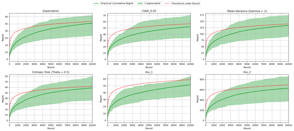
 -armed Bernoulli bandit, with different risk functionals, even combinations of them:

 runs!)
 cm of 30 randomly chosen students, I obtained the following data:
![\mu = \mathbb E[X]](https://s0.wp.com/latex.php?latex=%5Cmu+%3D+%5Cmathbb+E%5BX%5D&bg=ffffff&fg=000&s=0&c=20201002) .
. 
 and
and  . Assume
  holds, so that
  . Since
  , by the central limit theorem,
 :
:
 :
:

 , so that using either a
  – or a
  and the significance level
  .
. .
. .
. or
or  , it is true that
  . Therefore, there is sufficient evidence to reject
  cm.
cm. . Use the
 . Therefore,

 -confidence interval for
  , let
, let  denote the corresponding computed unbiased estimators for
  respectively. Then the computed corresponding confidence interval
  will equal
 , mimicking the computation above yields
 be a Bernoulli random variable that represents the gender of a person. Here
  denotes that the person is a man and
  denotes that the person is a woman. Denote
 ![p := \mathbb E[\xi]](https://s0.wp.com/latex.php?latex=p+%3A%3D+%5Cmathbb+E%5B%5Cxi%5D&bg=ffffff&fg=000&s=0&c=20201002) , which yields the proportion of women in the café.
, which yields the proportion of women in the café.
 . We next estimate
  using
using  :
:
 and
and  , by the central limit theorem,

 , which holds. Therefore, there is sufficient evidence to reject
  , let
, let  denote the number of students who scored
  marks out of 10. We have the following data:
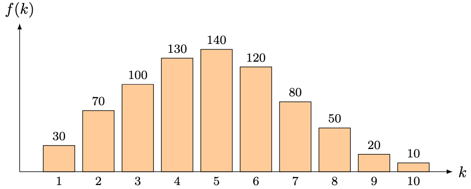
 . We first set up the null and alternative hypotheses:


 . Denoting

 -distribution with
  degrees of freedom. For a proof for why this distribution works, refer to
  (rounded to the nearest integer for readability, but whose original value we use in the final computation):

 , which does not hold. Therefore, there is (woefully) insufficient evidence to reject
 :
:
 . Therefore, there is sufficient evidence to reject
  , which implies
  .
. , for any
  ,
,
 , if
, if
 ,
,![\mathbb E[X] = 1/\lambda](https://s0.wp.com/latex.php?latex=%5Cmathbb+E%5BX%5D+%3D+1%2F%5Clambda&bg=ffffff&fg=000&s=0&c=20201002) ,
, ,
, of
of  is given by

![\begin{aligned} \mathbb E[X] &= \int_{-\infty}^{\infty} x f_X(x)\, \mathrm dx \\ &= \int_{0}^{\infty} \int_0^x f_X(x)\, \mathrm dy\, \mathrm dx \\ &= \int_{0}^{\infty} \int_{y}^\infty f_X(x) \, \mathrm dx \, \mathrm dy \\ &= \int_{0}^{\infty} \mathbb P(X > y) \, \mathrm dy. \end{aligned}](https://s0.wp.com/latex.php?latex=%5Cbegin%7Baligned%7D+%5Cmathbb+E%5BX%5D+%26%3D+%5Cint_%7B-%5Cinfty%7D%5E%7B%5Cinfty%7D+x+f_X%28x%29%5C%2C+%5Cmathrm+dx+%5C%5C+%26%3D+%5Cint_%7B0%7D%5E%7B%5Cinfty%7D+%5Cint_0%5Ex+f_X%28x%29%5C%2C+%5Cmathrm+dy%5C%2C+%5Cmathrm+dx+%5C%5C+%26%3D+%5Cint_%7B0%7D%5E%7B%5Cinfty%7D+%5Cint_%7By%7D%5E%5Cinfty+f_X%28x%29+%5C%2C+%5Cmathrm+dx+%5C%2C+%5Cmathrm+dy+%5C%5C+%26%3D+%5Cint_%7B0%7D%5E%7B%5Cinfty%7D+%5Cmathbb+P%28X+%3E+y%29+%5C%2C+%5Cmathrm+dy.+%5Cend%7Baligned%7D&bg=ffffff&fg=000&s=0&c=20201002)
![\begin{aligned} \mathbb E[X] &= \int_{0}^{\infty} e^{-\lambda y}\, \mathrm dy = \frac 1{\lambda} \cdot [-e^{-\lambda y}]_0^\infty = \frac 1{\lambda} \cdot (0 - (-1)) = \frac 1{\lambda}. \end{aligned}](https://s0.wp.com/latex.php?latex=%5Cbegin%7Baligned%7D+%5Cmathbb+E%5BX%5D+%26%3D+%5Cint_%7B0%7D%5E%7B%5Cinfty%7D+e%5E%7B-%5Clambda+y%7D%5C%2C+%5Cmathrm+dy+%3D+%5Cfrac+1%7B%5Clambda%7D+%5Ccdot+%5B-e%5E%7B-%5Clambda+y%7D%5D_0%5E%5Cinfty+%3D+%5Cfrac+1%7B%5Clambda%7D+%5Ccdot+%280+-+%28-1%29%29+%3D+%5Cfrac+1%7B%5Clambda%7D.+%5Cend%7Baligned%7D&bg=ffffff&fg=000&s=0&c=20201002)
![\begin{aligned} \mathbb E[X^2] &= \int_{-\infty}^{\infty} 2y \cdot \mathbb P(X > y) \, \mathrm dy \\ &= \int_{0}^{\infty} 2y \cdot e^{-\lambda y} \, \mathrm dy \\ &= \frac 2{\lambda} \int_0^\infty y e^{-\lambda y}\, \mathrm dy \\ &= \frac 2{\lambda} \cdot \mathbb E[X] = \frac 2{\lambda^2}. \end{aligned}](https://s0.wp.com/latex.php?latex=%5Cbegin%7Baligned%7D+%5Cmathbb+E%5BX%5E2%5D+%26%3D+%5Cint_%7B-%5Cinfty%7D%5E%7B%5Cinfty%7D+2y+%5Ccdot+%5Cmathbb+P%28X+%3E+y%29+%5C%2C+%5Cmathrm+dy+%5C%5C+%26%3D+%5Cint_%7B0%7D%5E%7B%5Cinfty%7D+2y+%5Ccdot+e%5E%7B-%5Clambda+y%7D+%5C%2C+%5Cmathrm+dy+%5C%5C+%26%3D+%5Cfrac+2%7B%5Clambda%7D+%5Cint_0%5E%5Cinfty+y+e%5E%7B-%5Clambda+y%7D%5C%2C+%5Cmathrm+dy+%5C%5C+%26%3D+%5Cfrac+2%7B%5Clambda%7D+%5Ccdot+%5Cmathbb+E%5BX%5D+%3D+%5Cfrac+2%7B%5Clambda%5E2%7D.+%5Cend%7Baligned%7D&bg=ffffff&fg=000&s=0&c=20201002)
![\displaystyle \mathrm{Var}(X) = \mathbb E[X^2] - \mathbb E[X]^2 = \frac{2}{\lambda^2} - \frac 1{\lambda^2} = \frac{1}{\lambda^2}.](https://s0.wp.com/latex.php?latex=%5Cdisplaystyle+%5Cmathrm%7BVar%7D%28X%29+%3D+%5Cmathbb+E%5BX%5E2%5D+-+%5Cmathbb+E%5BX%5D%5E2+%3D+%5Cfrac%7B2%7D%7B%5Clambda%5E2%7D+-+%5Cfrac+1%7B%5Clambda%5E2%7D+%3D+%5Cfrac%7B1%7D%7B%5Clambda%5E2%7D.&bg=ffffff&fg=000&s=0&c=20201002)

 is independent to
  .
. , evaluate the p.d.f. of
  .
. ,
,
 . To evaluate the p.d.f. of
  , we compute the convolution of their individual p.d.f.s:
 if it has a p.d.f. given by
 , then
 ![\mathbb E[X] = \alpha/\lambda](https://s0.wp.com/latex.php?latex=%5Cmathbb+E%5BX%5D+%3D+%5Calpha%2F%5Clambda&bg=ffffff&fg=000&s=0&c=20201002) ,
,  ,
, are i.i.d., then
  ,
, , then
  .
. . By definition of the expectation,
![\begin{aligned} \mathbb E[X^n] &= \int_0^\infty x^n \cdot \frac{\lambda^\alpha}{\Gamma(\alpha)} \cdot x^{\alpha - 1} \cdot e^{-\lambda x}\, \mathrm dx \\ &= \frac {\alpha \cdot (\alpha+1) \cdot \cdots \cdot (\alpha +n-1)}{\lambda^n} \cdot \int_0^\infty \frac{\lambda^{\alpha+n}}{\Gamma(\alpha+1)} \cdot x^{(\alpha + n) - 1} \cdot e^{-\lambda x}\, \mathrm dx \\ &= \frac{\alpha \cdot (\alpha+1) \cdot \cdots \cdot (\alpha +n-1)}{\lambda^n} \cdot \int_0^\infty f_Y(x)\, \mathrm dx \\ &= \frac{\alpha \cdot (\alpha+1) \cdot \cdots \cdot (\alpha +n-1)}{\lambda^n} . \end{aligned}](https://s0.wp.com/latex.php?latex=%5Cbegin%7Baligned%7D+%5Cmathbb+E%5BX%5En%5D+%26%3D+%5Cint_0%5E%5Cinfty+x%5En+%5Ccdot+%5Cfrac%7B%5Clambda%5E%5Calpha%7D%7B%5CGamma%28%5Calpha%29%7D+%5Ccdot+x%5E%7B%5Calpha+-+1%7D+%5Ccdot+e%5E%7B-%5Clambda+x%7D%5C%2C+%5Cmathrm+dx+%5C%5C+%26%3D+%5Cfrac+%7B%5Calpha+%5Ccdot+%28%5Calpha%2B1%29+%5Ccdot+%5Ccdots+%5Ccdot+%28%5Calpha+%2Bn-1%29%7D%7B%5Clambda%5En%7D+%5Ccdot+%5Cint_0%5E%5Cinfty+%5Cfrac%7B%5Clambda%5E%7B%5Calpha%2Bn%7D%7D%7B%5CGamma%28%5Calpha%2B1%29%7D+%5Ccdot+x%5E%7B%28%5Calpha+%2B+n%29+-+1%7D+%5Ccdot+e%5E%7B-%5Clambda+x%7D%5C%2C+%5Cmathrm+dx+%5C%5C+%26%3D+%5Cfrac%7B%5Calpha+%5Ccdot+%28%5Calpha%2B1%29+%5Ccdot+%5Ccdots+%5Ccdot+%28%5Calpha+%2Bn-1%29%7D%7B%5Clambda%5En%7D+%5Ccdot+%5Cint_0%5E%5Cinfty+f_Y%28x%29%5C%2C+%5Cmathrm+dx+%5C%5C+%26%3D+%5Cfrac%7B%5Calpha+%5Ccdot+%28%5Calpha%2B1%29+%5Ccdot+%5Ccdots+%5Ccdot+%28%5Calpha+%2Bn-1%29%7D%7B%5Clambda%5En%7D+.+%5Cend%7Baligned%7D&bg=ffffff&fg=000&s=0&c=20201002)
![\begin{aligned} \mathrm{Var}(X) &= \mathbb E[X^2] - \mathbb E[X]^2 = \frac{\alpha \cdot (\alpha+1)}{\lambda^2} - \frac{\alpha^2}{\lambda^2} = \frac{\alpha}{\lambda^2}. \end{aligned}](https://s0.wp.com/latex.php?latex=%5Cbegin%7Baligned%7D+%5Cmathrm%7BVar%7D%28X%29+%26%3D+%5Cmathbb+E%5BX%5E2%5D+-+%5Cmathbb+E%5BX%5D%5E2+%3D+%5Cfrac%7B%5Calpha+%5Ccdot+%28%5Calpha%2B1%29%7D%7B%5Clambda%5E2%7D+-+%5Cfrac%7B%5Calpha%5E2%7D%7B%5Clambda%5E2%7D+%3D+%5Cfrac%7B%5Calpha%7D%7B%5Clambda%5E2%7D.+%5Cend%7Baligned%7D&bg=ffffff&fg=000&s=0&c=20201002)
 are independent. To evaluate the p.d.f. of
 . Inductively, if
 ,
,
 .
. , write
  if there exists a random variable
  and
and  .
. ,
, ,
, ,
,  ,
, , then
  .
. , since
  ,
,
 . If
. If  , then
 , a random variable
  satisfies the memoryless property if the following holds: for any
  ,
,
 and
and  in terms of
  .
. . By the definition of conditional probability,
 for some
  . In particular,
 , so that
 is said to follow a geometric distribution with success probability
  , if
, if


![\displaystyle \mathbb E[X] = \sum_{x = 0}^\infty \mathbb P(X > x)](https://s0.wp.com/latex.php?latex=%5Cdisplaystyle+%5Cmathbb+E%5BX%5D+%3D+%5Csum_%7Bx+%3D+0%7D%5E%5Cinfty+%5Cmathbb+P%28X+%3E+x%29&bg=ffffff&fg=000&s=0&c=20201002) . Hence, evaluate
. Hence, evaluate ![\mathbb E[X]](https://s0.wp.com/latex.php?latex=%5Cmathbb+E%5BX%5D&bg=ffffff&fg=000&s=0&c=20201002) and
and  .
.![\begin{aligned} \mathbb E[X] &= \sum_{x = 0}^\infty x \cdot \mathbb P(X = x) \\ &= \sum_{x=0}^\infty \sum_{y=0}^{x-1} \mathbb P(X = x) \\ &= \sum_{y=0}^\infty \sum_{x=y+1}^\infty \mathbb P(X = x) \\ &= \sum_{y=0}^\infty \mathbb P(X > y) = \sum_{x = 0}^\infty \mathbb P(X > x). \end{aligned}](https://s0.wp.com/latex.php?latex=%5Cbegin%7Baligned%7D+%5Cmathbb+E%5BX%5D+%26%3D+%5Csum_%7Bx+%3D+0%7D%5E%5Cinfty+x+%5Ccdot+%5Cmathbb+P%28X+%3D+x%29+%5C%5C+%26%3D+%5Csum_%7Bx%3D0%7D%5E%5Cinfty+%5Csum_%7By%3D0%7D%5E%7Bx-1%7D+%5Cmathbb+P%28X+%3D+x%29+%5C%5C+%26%3D+%5Csum_%7By%3D0%7D%5E%5Cinfty+%5Csum_%7Bx%3Dy%2B1%7D%5E%5Cinfty+%5Cmathbb+P%28X+%3D+x%29+%5C%5C+%26%3D+%5Csum_%7By%3D0%7D%5E%5Cinfty+%5Cmathbb+P%28X+%3E+y%29+%3D+%5Csum_%7Bx+%3D+0%7D%5E%5Cinfty+%5Cmathbb+P%28X+%3E+x%29.+%5Cend%7Baligned%7D&bg=ffffff&fg=000&s=0&c=20201002)
![\displaystyle \mathbb E[X] = \sum_{x=0}^\infty (1-p)^x = \frac{1}{1-(1-p)} = \frac 1p.](https://s0.wp.com/latex.php?latex=%5Cdisplaystyle+%5Cmathbb+E%5BX%5D+%3D+%5Csum_%7Bx%3D0%7D%5E%5Cinfty+%281-p%29%5Ex+%3D+%5Cfrac%7B1%7D%7B1-%281-p%29%7D+%3D+%5Cfrac+1p.&bg=ffffff&fg=000&s=0&c=20201002)
![\mathbb E[X^2]](https://s0.wp.com/latex.php?latex=%5Cmathbb+E%5BX%5E2%5D&bg=ffffff&fg=000&s=0&c=20201002) . Observe that
. Observe that
![\begin{aligned} \mathbb E[X^2] &= \sum_{x = 0}^\infty x^2 \cdot \mathbb P(X = x) \\ &= \sum_{x=0}^\infty \sum_{y=0}^{x-1} (2y + 1) \cdot \mathbb P(X = x) \\ &= \sum_{y=0}^\infty \sum_{x=y+1}^\infty (2y + 1) \cdot \mathbb P(X = x) \\ &= \sum_{y=0}^\infty \left( (2y + 1) \cdot \sum_{x=y+1}^\infty (1-p)^{x-1} \cdot p \right) \\ &= \sum_{y=0}^\infty \left( (2y + 1) \cdot \frac{(1-p)^y}{1 - (1-p)} \cdot p \right) \\ &= \frac 1p \cdot \sum_{y=0}^\infty \left( (2y + 1) \cdot (1-p)^y \cdot p \right) \\ &= \frac 1p \cdot \left( p + (1-p) \cdot \left( 2 \cdot \sum_{y=1}^\infty y\cdot \mathbb P(X = y ) + \sum_{y=1}^\infty \mathbb P(X = y ) \right) \right) \\ &= \frac 1p \cdot \left( p + (1-p) \cdot \left( \frac 2p + 1 \right) \right) \\ &= 1 + \left( \frac 1p - 1 \right) \cdot \left( \frac 2p + 1 \right) \\ &= 1 + \frac 2{p^2} + \frac 1p - \frac 2p - 1 = \frac {2-p}{p^2}. \end{aligned}](https://s0.wp.com/latex.php?latex=%5Cbegin%7Baligned%7D+%5Cmathbb+E%5BX%5E2%5D+%26%3D+%5Csum_%7Bx+%3D+0%7D%5E%5Cinfty+x%5E2+%5Ccdot+%5Cmathbb+P%28X+%3D+x%29+%5C%5C+%26%3D+%5Csum_%7Bx%3D0%7D%5E%5Cinfty+%5Csum_%7By%3D0%7D%5E%7Bx-1%7D+%282y+%2B+1%29+%5Ccdot+%5Cmathbb+P%28X+%3D+x%29+%5C%5C+%26%3D+%5Csum_%7By%3D0%7D%5E%5Cinfty+%5Csum_%7Bx%3Dy%2B1%7D%5E%5Cinfty+%282y+%2B+1%29+%5Ccdot+%5Cmathbb+P%28X+%3D+x%29+%5C%5C+%26%3D+%5Csum_%7By%3D0%7D%5E%5Cinfty+%5Cleft%28+%282y+%2B+1%29+%5Ccdot+%5Csum_%7Bx%3Dy%2B1%7D%5E%5Cinfty+%281-p%29%5E%7Bx-1%7D+%5Ccdot+p+%5Cright%29+%5C%5C+%26%3D+%5Csum_%7By%3D0%7D%5E%5Cinfty+%5Cleft%28+%282y+%2B+1%29+%5Ccdot+%5Cfrac%7B%281-p%29%5Ey%7D%7B1+-+%281-p%29%7D+%5Ccdot+p+%5Cright%29+%5C%5C+%26%3D+%5Cfrac+1p+%5Ccdot+%5Csum_%7By%3D0%7D%5E%5Cinfty+%5Cleft%28+%282y+%2B+1%29+%5Ccdot+%281-p%29%5Ey+%5Ccdot+p+%5Cright%29+%5C%5C+%26%3D+%5Cfrac+1p+%5Ccdot+%5Cleft%28+p+%2B+%281-p%29+%5Ccdot++%5Cleft%28+2+%5Ccdot+%5Csum_%7By%3D1%7D%5E%5Cinfty+y%5Ccdot+%5Cmathbb+P%28X+%3D+y+%29++%2B+%5Csum_%7By%3D1%7D%5E%5Cinfty+%5Cmathbb+P%28X+%3D+y+%29++%5Cright%29+%5Cright%29+%5C%5C+%26%3D+%5Cfrac+1p+%5Ccdot+%5Cleft%28+p+%2B+%281-p%29+%5Ccdot++%5Cleft%28+%5Cfrac+2p++%2B+1+%5Cright%29+%5Cright%29+%5C%5C+%26%3D+1+%2B+%5Cleft%28+%5Cfrac+1p+-+1+%5Cright%29+%5Ccdot+%5Cleft%28+%5Cfrac+2p++%2B+1+%5Cright%29+%5C%5C+%26%3D+1+%2B+%5Cfrac+2%7Bp%5E2%7D+%2B+%5Cfrac+1p+-+%5Cfrac+2p+-+1+%3D+%5Cfrac+%7B2-p%7D%7Bp%5E2%7D.+%5Cend%7Baligned%7D&bg=ffffff&fg=000&s=0&c=20201002)
![\begin{aligned} \mathrm{Var}(X) &= \mathbb E[X^2] -\mathbb E[X]^2 = \frac {2-p}{p^2} - \frac 1{p^2} = \frac{1-p}{p^2}. \end{aligned}](https://s0.wp.com/latex.php?latex=%5Cbegin%7Baligned%7D+%5Cmathrm%7BVar%7D%28X%29+%26%3D+%5Cmathbb+E%5BX%5E2%5D+-%5Cmathbb+E%5BX%5D%5E2+%3D+%5Cfrac+%7B2-p%7D%7Bp%5E2%7D+-+%5Cfrac+1%7Bp%5E2%7D+%3D+%5Cfrac%7B1-p%7D%7Bp%5E2%7D.+%5Cend%7Baligned%7D&bg=ffffff&fg=000&s=0&c=20201002)
 is independent of
  . Then
 .
. . For any

